Abstract. Snow on Antarctic sea ice strongly influences the thermodynamics and freshwater balance of the coupled sea ice–upper ocean system. Yet understanding of its temporal and spatial variations remains limited by sparse observations, large uncertainties in remote sensing retrievals, and idealized model representations. We introduce a new open-source numerical model, the University of Washington Snow on Antarctic Ice Lagrangian (WASSAIL) model, that simulates the mass and bulk density evolution of snow on sea ice in the Southern Ocean over 2003–2025. Hourly reanalysis snowfall is accumulated along Lagrangian sea ice drift trajectories determined from remotely sensed ice motion fields. The single-layer model incorporates physically and empirically informed parameterizations of key erosion and transformation processes, including surface and wind-blown snow sublimation, lead trapping, rain- and non-rain-related melt, compaction from wind and overburden pressure, and the large-scale effects of sea ice convergence and divergence. Model parameters are calibrated using snow buoy measurements from the Weddell Sea. The resulting reconstruction indicates that over one-third of annual snowfall intercepted by Antarctic sea ice is lost to the atmosphere, ocean, or to melt processes prior to complete sea ice melt, with blowing snow sublimation as the dominant sink. Comparison with satellite snow depth retrievals further suggests that widespread snow-ice formation consumes 49–60 % of the remaining snow. Overall, we infer an annual meteoric freshwater input to the Southern Ocean originating from snow on sea ice of 237 mSv, equivalent to more than half of the freshwater flux associated with circumpolar sea ice melt.
Scientific programming has become increasingly essential for manipulating, visualizing, and interpreting the large volumes of data acquired in earth science research. Yet few discipline-specific instructional approaches have been documented and assessed for their effectiveness in equipping geoscience undergraduate students with coding skills. Here we report on an evidence-based redesign of an introductory Python programming course, taught fully remotely in 2020 in the School of Oceanography at the University of Washington. Key components included a flipped structure, synchronous activities infused with active learning, an individualized final research project, and a focus on creating an accessible learning environment. Cloud-based notebooks were used to teach fundamental Python syntax as well as functions from packages widely used in climate-related disciplines. By analyzing quantitative and qualitative data from surveys, online learning platforms, student work, assessments, and a focus group, we conclude that the instructional design facilitated learning and supported self-guided scientific inquiry. Students with less or no prior exposure to coding achieved similar success to peers with more previous experience, an outcome likely mediated by higher engagement with course resources. We believe that the constructivist approach to teaching introductory programming and data literacy that we present could be broadly applicable across the earth sciences and in other scientific domains.
In the frequency band of 1–20 kHz, wind-generated breaking surface waves produce bubbles near the surface that are the dominant ambient noise source. In previous work, two decades of ambient noise data from six deep ocean moorings were used to validate ambient noise models (Yang et al., JASA EL 3(3), 2023). Data-model comparisons show a mismatch, as existing models are monotonic in nature, i.e., the modeled spectral level increases with increasing wind speed for all frequencies, while data display a sharp drop-off that creates a “cross-over” as the spectral level for wind speed exceeding 15 m/s and frequency above ∼4 kHz becomes lower than that at lower wind speeds. This mismatch is due to attenuation when ambient sound propagates through the deeper and denser bubble layer under high sea conditions. In this work, an empirical ambient noise model utilizing wind speed only is presented as a baseline prediction with potential fine-tuning parameters such as bubble statistics, current and its direction, and wave height discussed. [Work supported by NOAA, NASA, and ONR.]
Seasonal patterns in seasonally frozen waters have usually been derived from composites of analyses conducted in different years and largely have been confined to ice-free periods. We present the first continuous measurements of hydrographic and biogeochemical variables collected over an entire year by Biogeochemical-Argo (BGC-Argo) profiling floats on the continental shelf of the Ross Sea. Analyses were divided into two periods: autumn/winter and spring/summer. Mixed layers increased rapidly upon ice cover, and nitrate, oxygen, and dissolved inorganic carbon vertical distributions were strongly influenced by this deeper mixing. Rates of nitrification in autumn were substantial and similar to rates measured in other areas of the ocean. Organic carbon disappearance was also most rapid in March. Changes in all variables slowed considerably after May. The largest mixed layer depths occurred at the southern floats and reached 400 - 500 m. Spring/summer patterns were similar to those observed during individual cruises, with rapid nitrate removal beginning in November, continuing through early January, but ceasing during austral summer. The most rapid accumulations of chlorophyll occurred prior to complete ice retreat. Substantial spatial differences were noted that were likely related to both mixed layer depths and phytoplankton composition. Particulate matter accumulated throughout the summer below 100 m, although the rates of change suggested substantial remineralization in the water column. The temporal patterns observed show the importance of relatively short periods that markedly influence the vertical distribution of biogeochemical parameters.
The distinctive underwater sound generated by raindrops on the ocean surface has been used to detect and quantify rainfall. Knowledge of the intensity and spatial–temporal distribution of rainfall over the ocean is critical in understanding the global hydrological cycle. However, rainfall is difficult to measure accurately over the ocean due to its spatial and temporal variability. To reduce these problems, satellite-based rain-monitoring instruments are used but they do not capture the full in situ temporal and spatial variability. The Passive Aquatic Listener (PAL) was developed at the University of Washington’s Applied Physics Laboratory (Nystuen, J. Acoust. Soc. 79, 92–98). PAL has been incorporated into Argo floats and deployed over global oceans. PAL-Argos are capable of telemetering back estimated rain rate and wind speed with a temporal resolution of 2–8 min, representing a circular surface footprint of a few kilometer radius (Yang et al., Oceanography 28, 124–133). In this work, the major operations of PAL-Argos in NASA’s Aquaris Satellite Mission, SPURS field efforts related to the Tropical Rainfall Measuring Mission, NOAA’s Tropical Pacific Observing System Initiative, and NSF’s Measurements and Modelling of the Indonesian Throughflow are chronicled with selective field data presented. [Work supported by NASA, NOAA, and NSF.]
The Sea of Okhotsk is a marginal sea that plays a major role in the ventilation of the North Pacific, being the key location where Dense Shelf Water (DSW) forms at the surface and sinks to the intermediate layer. The Okhotsk Sea Intermediate Water (OSIW) is a key water mass because it includes large amounts of DSW, outflows to the North Pacific, and supplies the ocean with the micronutrient iron. OSIW has been warming over the past few decades, which is attributed to a decreasing trend in DSW production. The acquisition of numerous hydrographic data after 2000 in the Kuril Basin, especially dissolved oxygen from profiling floats, offers an opportunity to better quantify the water mass composition of OSIW, and the changes in OSIW properties and DSW volume. Here, we used all available hydrographic records and a mapping technique specially adapted to polar and sub-polar regions to revisit the Sea of Okhotsk water properties and document their long-term changes. Our analysis revealed that the volume of heavier DSW (potential density above 26.9 kg.m-3) has decreased over the past three decades by 3,600 km3, or 15% of the volume present before 1990. This decline is nearly entirely compensated for by an increase in lighter DSW. This shift toward lighter DSW is possibly a sign of the weakening of the intermediate overturning circulation starting in the Okhotsk Sea. Additionally, we found that dense Soya Current Water only accounts for about 1% of OSIW, against the 5% previously estimated. The water of the Sea of Okhotsk is a mix of several water masses which includes the Dense Shelf Water (DSW), a water mass generated in winter via sea ice formation. When sea ice forms, the surface water salinity and density increase, and the cold DSW is generated as the surface water sinks to the bottom of the continental shelf while micronutrients, especially iron, are also incorporated. DSW mixes with other water masses and becomes the Okhotsk Sea Intermediate Water (OSIW) before being exported to the North Pacific where it plays an important role for both the climate and the biological productivity. In this study, we used all the temperature, salinity, and dissolved oxygen data acquired since 1930 to evaluate how global warming may have affected the composition of OSIW. We found that, over the past century, the amount of denser DSW has strongly decreased whereas that of lighter DSW has increased, which is consistent with the decline in sea ice production in the Sea of Okhotsk. This also suggests that the ventilation of the Sea of Okhotsk and the circulation of the intermediate layer of the North Pacific is weakening, which could indirectly affect the ocean's biological productivity. The composition of the Okhotsk Sea Intermediate Water (OSIW) is reevaluated using an updated data set and a new mapping technique OSIW properties have changed in the long-term (>= 50 years) scale, with a decrease (increase) in the amount of heavy (light) Dense Shelf Water This suggests that the North Pacific intermediate overturning is weakening, which could affect the ocean's biological productivity
This study provides the first estimation of sea ice-melt amount in the Sea of Okhotsk based on spring hydrographic data accumulated for nearly a hundred years. Just after sea ice melts completely, a low-salinity layer appears on the ocean surface, overlying the layer of Winter Water at the freezing point. The integration of the salinity decrease from Winter Water should correspond to the total ice-melt amount. We developed an algorithm to extract the profiles that clearly show the salinity deficit and converted the salinity deficit to the ice-melt amount from all available data. The climatological map shows that ice-melt amount decreases toward the ice edge and exhibits large values around the northern Sakhalin Island, reflecting the ice thickness distribution. In the southern area (south of 48°N), where sea ice is transported from the north, the average ice-melt amount is estimated to be 71 cm in thickness. It is clearly shown that the ice-melt amount has decreased by 30
Global estimates of mesoscale vertical velocity remain poorly constrained due to a historical lack of adequate observations on the spatial and temporal scales needed to measure these small magnitude velocities. However, with the wide-spread and frequent observations collected by the Argo array of autonomous profiling floats, we can now better quantify mesoscale vertical velocities throughout the global ocean. We use the underutilized trajectory data files from the Argo array to estimate the time evolution of isotherm displacement around a float as it drifts at 1,000 m, allowing us to quantify vertical velocity averaged over approximately 4.5 days for that depth level. The resulting estimates have a non-normal, high-peak, and heavy-tail distribution. The vertical velocity distribution has a mean value of (1.9 +/- 0.02) x 10-6 m s-1 and a median value of (1.3 +/- 0.2) x 10-7 m s-1, but the high-magnitude events can be up to the order of 10-4 m s-1. We find that vertical velocity is highly spatially variable and is largely associated with a combination of topographic features and horizontal flow. These are some of the first observational estimates of mesoscale vertical velocity to be taken across such large swaths of the ocean without assumptions of uniformity or reliance on horizontal divergence. Vertical velocity in the ocean is a fundamental part of how water circulates throughout the globe. This impacts the temperature, salt, nutrients, and currents that make up the ocean. However, vertical velocities are very small and are, therefore, difficult to measure. In particular, the vertical velocities of ocean events that occur on roughly a weekly to monthly time scale (mesoscale) are poorly understood. We have developed a method for estimating these mesoscale vertical velocities across the globe using an array of autonomous robots called Argo floats. Our results show that vertical velocities vary greatly depending on location, with the largest values occurring where there is a combination of relatively shallow ocean depths and larger horizontal velocities. These estimates are some of the first of their kind to be made from observations across such large swaths of the ocean. Five-day averaged vertical velocities from Argo observations near 1,000 m are non-normally distributed, with a high peak and heavy tailsMesoscale vertical velocities are on the order of centimeters per day, but high-magnitude events can be on the order of meters per dayVertical velocities estimated from Argo floats are spatially variable and correlated with topographic features and horizontal surface flow
Bubbles from wind generated breaking surface waves are the dominant ambient noise source [Dean and Stokes, Nature 418, 839-844 (2002)]. With ambient noise data collected in the open ocean between 100 Hz and 50 kHz from 1999 to 2022, the ambient noise level is observed to sharply decrease as wind speed increases beyond 15 m/s for frequencies higher than 4 kHz. Data-model comparisons show a mismatch, as existing models including the Wenz curves [Wenz, J. Acoust. Soc. Am. 34, 1936-1956 (1962)] are monotonic in nature. The decrease at high wind speeds and frequencies is likely due to attenuation when ambient sound propagates through the deeper and denser bubble layer for high sea conditions [Farmer and Lemon, J. Phys. Oceanogr. 14, 1761-1777 (1984)].
In recent years, the Southern Ocean has experienced unprecedented surface warming and sea ice loss}a stark reversal of the sea ice expansion and surface cooling that prevailed over the preceding decades. Here, we examine the mechanisms that led to the abrupt circumpolar surface warming events that occurred in late 2016 and 2019 and assess the role of internal climate variability. A mixed layer heat budget analysis reveals that these recent circumpolar surface warming events were triggered by a weakening of the circumpolar westerlies, which decreased northward Ekman transport and accelerated the seasonal shoaling of the mixed layer. We emphasize the underappreciated effect of the latter mechanism, which played a dominant role and amplified the warming effect of air-sea heat fluxes during months of peak solar insolation. An examination of the CESM1 large ensemble demonstrates that these recent circumpolar warming events are consistent with the internal variability associated with the Southern Annular Mode (SAM), whereby negative SAM in austral spring favors shallower mixed layers and anomalously high summertime SST. A key insight from this analysis is that the seasonal phasing of springtime mixed layer depth shoaling is an important contributor to summertime SST variability in the Southern Ocean. Thus, future Southern Ocean summertime SST extremes will depend on the coevolution of mixed layer depth and surface wind variability.
Rain over the ocean is a central process in the global freshwater cycle. The freshening of the ocean surface due to rain can be seen in global maps of sea surface salinity, where areas with high precipitation are broadly coincident with areas of low salinity and regions of high salinity occur in regions with low precipitation and high evaporation. The transfer of water from these evaporating regions to the precipitating regions drives the global water cycle, and understanding its dynamics is essential in determining how weather patterns will respond to changes in global climate. Rain is difficult to measure over the ocean due to its spatial and temporal variability and the limitations imposed by rain gauges when mounted on moving platforms. However, the loud and distinctive underwater sound generated by raindrops on the ocean surface can be used to detect and quantify rainfall and to track climate change impacts. The work here will focus on deriving time series of rain rate with temporal resolution on the order of minutes using ambient noise recorded by Passive Aquatic Listener (PAL) on both Argo floats and deep ocean moorings (Nystuen, J., Atmos. Oceanic Tech, 13, 74–84, 1996). [Work supported by NOAA and NASA.]
Net community production (NCP) was estimated from nitrate profiles measured via biogeochemical Argo floats drifting in the Argentine Basin. Two criteria were tested for defining hydrographic fronts used to separate the study area into five zones: potential density anomaly at 450 m and potential temperature at 100 m. The latter definition was preferred as it minimized overlapping among zones. Float profiles within each zone were used to construct monthly median profiles of nitrate. Monthly nitrate inventories were calculated for each zone by integrating the median profiles between the surface and a depth of 100 or 200 m. Three methods were utilized to estimate NCP from the nitrate drawdown. The resulting mean NCP estimates indicated a decline in NCP from 3 to 4 mol Cm-2 yr(-1) south of similar to 40 degrees S to <= 1 mol Cm-2 yr(-1) north of similar to 40 degrees S. The monthly median profiles suggested 20%-100% of drawdown occurred by the end of December; however, chlorophyll fluorescence indicated phytoplankton activity persisted through austral summer. We speculate that primary production during these summer months was supported by regenerated nitrogen sources (not nitrate), despite replete concentrations, likely due to the relative scarcity of bioavailable iron known to persist in the region. While a northward advective flux of nitrate was strongly suggested by meridional nitrate gradients over the upper 0-300 m, vertical mixing was apparently necessary to stimulate new production, indicating both processes are important for NCP in the Argentine Basin. This work highlights the potential for floats in studying biogeochemical cycles in hydrographically complex regions.
Ocean ambient noise, spanning from a few hertz to tens of kilohertz, is often the limiting factor for sonar performance in target detection, location, and identification. In this frequency band, wind generated surface breaking waves produce bubbles near the surface that are the dominant ambient noise source. In this work, results from a long-term collaboration between NOAA/ NASA and ambient noise study pioneer, Jeffrey A. Nystuen, are presented. Specifically, two-decades of ambient noise data from six deep ocean moorings with companion surface meteorological measurements are used to validate ambient noise models. Excluding data during rainy periods, the ambient noise level is investigated under different wind speed ranges. For wind speeds exceeding 15 m/s, the ambient noise level displays a sharp drop-off and creates a “cross-over” as the spectral level at higher wind speeds and frequencies becomes lower than that at lower wind speeds. Data-model comparisons show a mismatch, as existing models are monotonic in nature, i.e., the modeled spectral level increases with increasing wind speed for all frequencies. This mismatch, currently under investigation, is likely due to attenuation when ambient sound propagates through the deeper and denser bubble layer under high sea conditions. [Work supported by NOAA, NASA, and ONR.]
The Southern Ocean serves as the primary gateway through which the intermediate, deep, and bottom waters of the ocean interact with the surface ocean (and thus the atmosphere), and it has a profound influence on the oceanic uptake of anthropogenic carbon and heat as well as nutrient resupply from the abyss to the surface. Yet it has been the least observed and understood region of the world ocean. The Southern Ocean Carbon and Climate Observations and Modeling (SOCCOM) project was implemented in 2014 with a goal to help remedy this deficit in observations and understanding. The SOCCOM project is based on two major advances that have the potential to transform understanding of the Southern Ocean. The first is the development of new biogeochemical sensors mounted on autonomous profiling floats that allow sampling of ocean biogeochemistry in 3-dimensional space. Floats may detect processes with a temporal resolution that ranges from hours to years. The second is that the climate modeling community finally has the computational resources and physical understanding to develop fully coupled climate models that can represent crucial, mesoscale processes in the Southern Ocean, as well as corresponding models that assimilate observations to produce a state estimate. The observational component, based on deployment of profiling floats with oxygen, nitrate, pH and bio-optical sensors, is generating vast amounts of new biogeochemical data that provide a year-round view of the Southern Ocean from the surface to 2000 m. The modeling effort is applying these observations and enhancing our understanding of the current ocean, and reducing uncertainty in projections of future carbon and nutrient cycles and climate. After nine years of operation, including a project renewal in the sixth year, the SOCCOM project has deployed more than 260 profiling floats. These floats have collected over 27,000 vertical profiles throughout the Southern Ocean. A data assimilating biogeochemical state estimate model has been implemented. Here, the design of the SOCCOM project is reviewed and the scientific results that have been obtained are described. The project's capability to help meet the observing system priorities outlined for a notional UN Decade for Ocean Sciences Southern Ocean observing system is assessed.
Global estimates of mesoscale vertical velocity remain poorly constrained due to a historical lack of adequate observations on the spatial and temporal scales needed to measure these small magnitude velocities. However, with the wide-spread and frequent observations collected by the Argo array of autonomous profiling floats, we can now better quantify mesoscale vertical velocities throughout the global ocean. We use the underutilized trajectory data from the Argo array to estimate the time evolution of isotherm displacement around a float as it drifts at 1000 dbar, allowing us to quantify vertical velocity averaged over approximately 4.5 days for that pressure level. The resulting estimates have a non-normal, high-peak, and heavy-tail distribution. The vertical velocity distribution has a mean value of (1.9±0.02)×10-6 m s-1 and a median value of (1.3± 0.2)×10-7 m s-1, but the high-magnitude events can be up to the order of 10−4 m s-1 , We find that vertical velocity is highly spatially variable and is largely associated with a combination of topographic features and horizontal flow. These are some of the first observational estimates of mesoscale vertical velocity to be taken across such large swaths of the ocean without assumptions of uniformity or reliance on horizontal divergence.
Despite its importance for the global cycling of carbon, there are still large gaps in our understanding of the processes driving annual and seasonal carbon fluxes in the high‐latitude Southern Ocean. This is due in part to a historical paucity of observations in this remote, turbulent, and seasonally ice‐covered region. Here, we use autonomous biogeochemical float data spanning 6 full seasonal cycles and with circumpolar coverage of the Southern Ocean, complemented by atmospheric reanalysis, to construct a monthly climatology of the mixed layer budget of dissolved inorganic carbon (DIC). We investigate the processes that determine the annual mean and seasonal cycle of DIC fluxes in two different zones of the Southern Ocean—the Sea Ice Zone (SIZ) and Antarctic Southern Zone (ASZ). We find that, annually, mixing with carbon‐rich waters at the base of the mixed layer supplies DIC which is, in the ASZ, either used for net biological production or outgassed to the atmosphere. In contrast, in the SIZ, where carbon outgassing and the biological pump are weaker, the surplus of DIC is instead advected northward to the ASZ. In other words, carbon outgassing in the southern Antarctic Circumpolar Current (ACC), which has been attributed to remineralized carbon from deep water upwelled in the ACC, is also due to the wind‐driven transport of DIC from the SIZ. These results stem from the first observation‐based carbon budget of the circumpolar Southern Ocean and thus provide a useful benchmark to evaluate climate models, which have significant biases in this region.
Acoustically tracked subsurface floats provide insights into ocean complexity and were first deployed over 60 years ago. A standard tracking method uses a Least-Squares algorithm to estimate float trajectories based on acoustic ranging from moored sound sources. However, infrequent or imperfect data challenge such estimates. Acoustic tracking is currently the only feasible strategy for recovering float positions in the sea ice region, a focus of this study. Acoustic records recovered from under-ice floats frequently lack continuous sound source coverage. This is because environmental factors such as surface sound channels and sea ice attenuate acoustic signals, while operational considerations make polar sound sources difficult to deploy. Here we present a Kalman Smoother approach that, by including some estimates of float behavior, extends tracking to situations with more challenging data sets. The Kalman Smoother constructs dynamically constrained, error-minimized float tracks using all possible position data. The Kalman Smoother is applied to previously-tracked floats from the southeast Pacific (DIMES experiment), and the results are compared with existing trajectories constructed using the Least-Squares algorithm. The Kalman Smoother is also used to reconstruct the trajectories of a set of previously untracked, acoustically-enabled Argo floats in the Weddell Sea.
Measurements of pH and nitrate from the Southern Ocean Carbon and Climate Observations and Modeling array of profiling floats were used to assess the ratios of dissolved inorganic carbon (DIC) and nitrate (NO3) uptake during the spring to summer bloom period throughout the Southern Ocean. Two hundred and forty-three bloom periods were observed by 115 floats from 30 degrees S to 70 degrees S. Similar calculations were made using the Takahashi surface DIC and nitrate climatology. To separate the effects of atmospheric CO2 exchange and mixing from phytoplankton uptake, the ratios of changes in DIC to nitrate of surface waters (Delta DIC/Delta NO3) were computed in the Biogeochemical Southern Ocean State Estimate (B-SOSE) model. Phytoplankton uptake of DIC and nitrate are fixed in B-SOSE at the Redfield Ratio (RR; 6.6 mol C/mol N). Deviations in the B-SOSE Delta DIC/Delta NO3 must be due to non-biological effects of CO2 gas exchange and mixing. Delta DIC/Delta NO3 values observed by floats and in the Takahashi climatology were corrected for the non-biological effects using B-SOSE. The corrected, in situ biological uptake ratio (C:N) occurs at values similar to the RR, with two major exceptions. North of 40 degrees S biological DIC uptake is observed with little or no change in nitrate giving high C:N. In the latitude band at 55 degrees S, the Takahashi data give a low C:N value, while floats are high. This may be due to a change in CO2 air-sea exchange in this region from uptake during the Takahashi reference year of 2005 to outgassing of CO2 during the years sampled by floats.
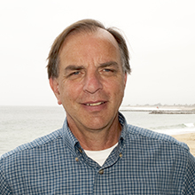 Ken Johnson合作论文数Monterey Bay Aquarium Research Institute60
 Lynne D. Talley合作论文数Scripps Institution of Oceanography, University of California, San Diego53
 Jorge Sarmiento合作论文数Department of Geosciences, Princeton University;Princeton Environmental Institute, Princeton University;Andlinger Center for Energy and The Environment, Princeton University31
 Dana D. Swift合作论文数20
 Nancy L. Williams合作论文数Rosenstiel School of Marine and Atmospheric Science, University of Miami18
 Joellen Louise Russell合作论文数Department of Geosciences, The University of Arizona18
 Emmanuel S. Boss合作论文数Maine In-situ Sound & Color Lab, School of Marine Sciences, University of Maine17Joshua N. Plant合作论文数15
 Dean Roemmich合作论文数Integrative Oceanography Division, Scripps Institution of Oceanography, University of California, San Diego;Climate, Atmospheric Science, and Physical Oceanography Division, Scripps Institution of Oceanography, University of California, San Diego15
 Matthew R. Mazloff合作论文数Scripps Institution of Oceanography, University of California15
 Annie P. S. Wong合作论文数University of Washington;NOAA;Woods Hole Oceanographic Institution;Woods Hole Oceanographic Institution, University of Washington14
 Gregory C. Johnson合作论文数Ocean Climate Research Division, Pacific Marine Environmental Laboratory, National Oceanic and Atmospheric Administration;School of Oceanography, University of Washington14Alison R. Gray合作论文数13Tanya L. Maurer合作论文数12Robert Key合作论文数Program in Atmospheric and Oceanic Sciences, Princeton University12
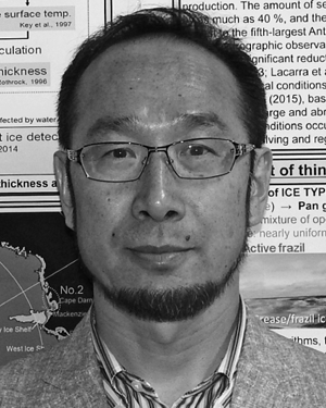 Kay I. Ohshima合作论文数12Luke J. Coletti合作论文数11
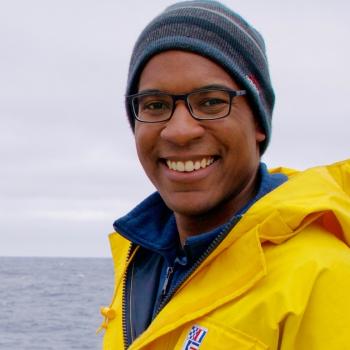 Earle Wilson合作论文数Department of Earth System Science, Doerr School of Sustainability, Stanford University10
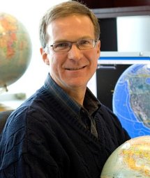 Denis Gilbert合作论文数Fisheries & Oceans Canada, Maurice Lamontagne Inst10
 Susan Wijffels合作论文数CSIRO10
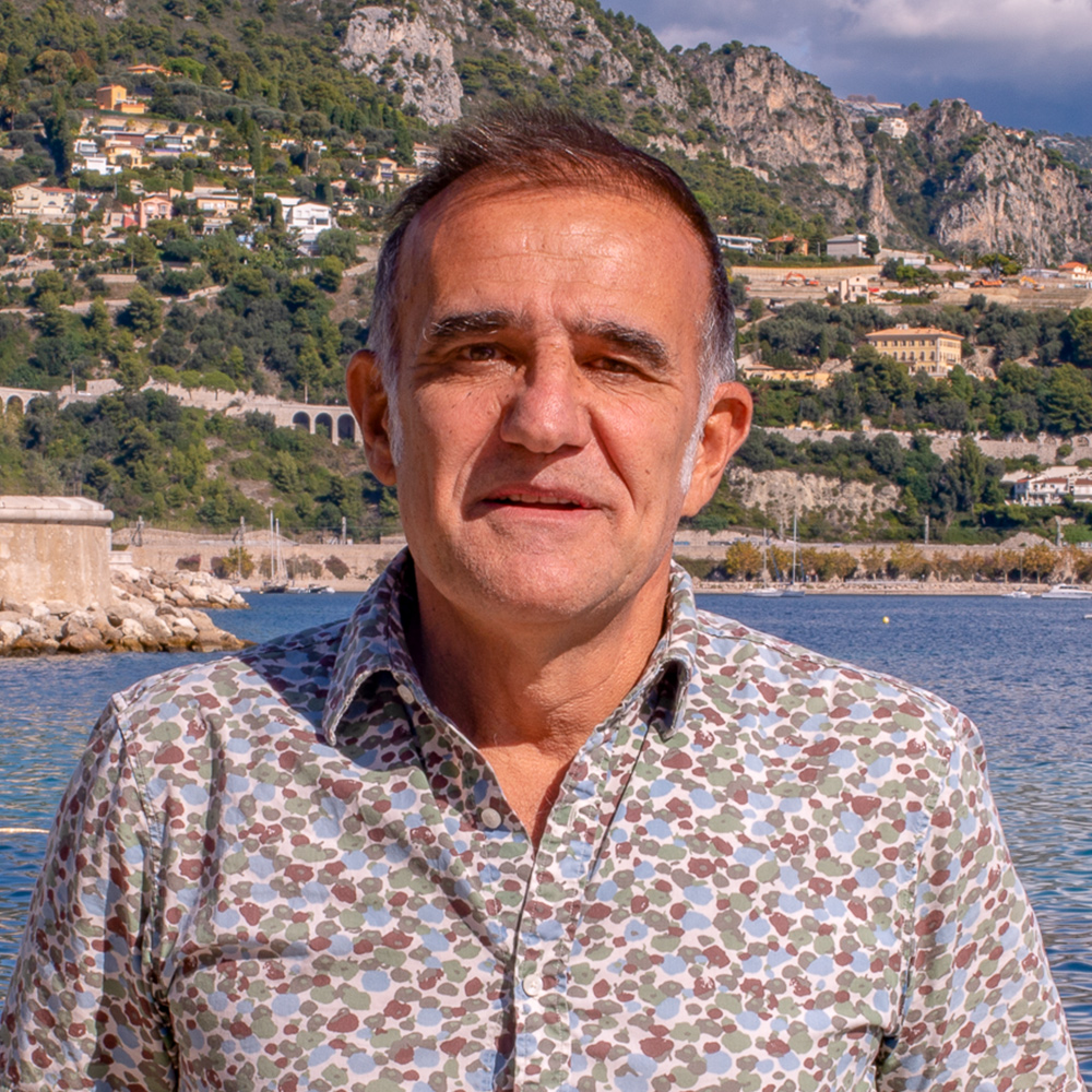 Herve Claustre合作论文数Laboratoire d'Oceanographie de Villefranche, CNRS;Sorbonne University10
 Richard (Rik) Wanninkhof合作论文数NOAA's Atlantic Oceanographic and Meteorological Laboratory, U.S. Department of Commerce9
 Virginie Thierry合作论文数9Richard H Wanninkhof合作论文数8
 Yang Jie合作论文数8
 Andrew Dickson合作论文数Scripps Institution of Oceanography, University of California, San Diego8
 Richard A. Feely合作论文数Pacific Marine Environmental Laboratory, National Oceanic and Atmospheric Administration;Department of Oceanography, University of Washington8Carole M. Sakamoto合作论文数8
 Kortzinger Arne合作论文数Leibniz Institute of Marine Sciences8
 Todd Martz合作论文数Scripps Institution of Oceanography, University of California, San Diego7Robert Drucker合作论文数7
 Steven R. Jayne合作论文数Climate and Global;Dynamics Division;National Center;Climate and Global, National Center7Hans W. Jannasch合作论文数7Roberta M. Hotinski合作论文数6
 Ethan C. Campbell合作论文数Univ Washington, Sch Oceanog, Seattle, WA 98195 USA6Bittig Henry合作论文数6
 Seth M. Bushinsky合作论文数Monterey Bay Aquarium Research Institute6
 Howard J. Freeland合作论文数Institute of Ocean Sciences6
 H. Thomas Rossby合作论文数Graduate School of Oceanography, University of Rhode Island6
 Katja Fennel合作论文数Department of Oceanography, Dalhousie University6
 Nathalie Zilberman合作论文数6A. R. Gray合作论文数5Philip Sutton合作论文数5
 Takeshita Yuichiro合作论文数5
 Vigan Mensah合作论文数5
 Toshio Suga合作论文数Graduate School of Science, Tohoku University5
 Takuya Nakanowatari合作论文数5Cesar Villanoy合作论文数Marine Science Institute, University of the Philippines5Kevin G. Speer合作论文数5




