Linear algebra is one of the most basic foundations of a wide range of scientific domains, and most textbooks of linear algebra are written by mathematicians. However, this book is specifically intended to students and researchers of pattern information processing, analyzing signals such as images and exploring computer vision and computer graphics applications. The author himself is a researcher of this domain.
The pseudoinverse introduced in the preceding chapter is closely related to the least-squares method for linear equations. In fact, the theory of pseudoinverse has been studied in relation to minimization of the sum of squares of linear equations. The least-squares method usually requires solving an equation, called the “normal equation,” obtained by letting the derivative of the sum of squares be zero. In this chapter, we show how a general solution is obtained without using differentiation or normal equations. As illustrative examples, we show the case of multiple equations of one variable and the case of a single multivariate equation.
In this chapter, we regard measurement data that conain noise not as definitive values but as “random variables” specified by probability distributions. The principal parameters that characterize a probability distribution are the “mean” (average) and the “covariance matrix.” In particular, the “normal” (or “Gaussian”) distribution is characterized by the mean and the covariance matrix alone. We show that if the probability is not distributed over the entire space but is restricted to some domain, e.g., constrained to be on a planar surface or on a sphere, the covariance matrix becomes singular. In such a case, the probability distribution is characterized by the pseudoinverse of the covariance matrix. We illustrate how this leads to a practical method for comparing computational accuracy of such data.
In this chapter, we show that a symmetric matrix can be expressed in terms of its “eigenvalues” and “eigenvectors.” This expression is called the “spectral decomposition” of a symmetric matrix. It allows us to convert a symmetric matrix into a diagonal matrix by multiplying it by an “orthogonal matrix” from left and right. This process is called “diagonalization” of a symmetric matrix. We can also express the inverse and powers of a symmetric matrix in terms of its spectral decomposition.
We study the SVD of an arbitrary matrix A nxm , especially its subspaces of activation, which leads in natural manner to pseudoinverse of Moore-Bjenhammar-Penrose. Besides, we analyze the compatibility of linear systems and the uniqueness of the corresponding solution, and our approach gives the Lanczos classification for these systems.
In this chapter, we generalize line fitting in 2D and plane fitting in 3D to general dimensions and consider how to fit subspaces and affine spaces to a given set of points in nD. A subspace is a space spanned by vectors starting from the origin, and an “affine space” is a translation of a subspace to a general position. The fitting is done hierarchically: we first fit a lower dimensional space, starting from a 0D space (= a point), then determine a space with an additional dimension so that the discrepancy is minimized, and continue this. This principle corresponds to what is known as “Karhunen-Loeve expansion” in signal processing and pattern recognition and as “principal component analysis” in statistics. The fitted space is computed from the spectral decomposition of a matrix, which we call the “covariance matrix,” but also can be obtained from its singular value decomposition. We point out that the use of the singular value decomposition is more efficient with smaller computational complexity.
In this chapter, we introduce the concepts of “projection” and “rejection” and express them in the form of the “projection matrix.” They play a central role in this book, because it implies both “orthogonality” and “shortest distance.” The themes of the subsequent chapters are all based on these two aspects of projection. First, we define “subspaces,” “orthogonal complements,” and “direct sum decomposition” and then derive concrete expressions of the projection matrix. As an illustration, we show examples of projection onto lines and planes and introduce the “Schmidt orthogonalization” for producing an orthonormal system of vectors using projection matrices.
This chapter describes the principles and procedure for computing the 3D position of a corresponding point pair between two images of a known planar surface by assuming knowledge of the camera matrices of the two cameras. This process is called planar triangulation. We first show that the homography between the two images is determined from the equation of the plane and the camera matrices. The principle of planar triangulation is to correct the corresponding point pair optimally such that the associated lines of sight intersect precisely at a point on the assumed plane, using knowledge of the statistical properties of image noise. It turns out that the procedure is closely related to the optimal homography computation described in the preceding chapter (Chap. 6 ).
This chapter describes the procedure for computing, from corresponding points between two images of a planar scene, the 3D position of that plane and the camera matrices of the two cameras that took those images. First, we express the matrix of the homography between the two images in terms of the 3D position of the plane and the two camera matrices. We then show how to decompose the homography matrix into the 3D position of the plane and the two camera matrices in an analytical form. The solution is not unique; we describe the procedure for selecting the correct one. Once the camera matrices are obtained, the 3D positions of the corresponding point pairs are computed by the planar triangulation procedure of the preceding chapter.
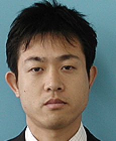 Yasuyuki Sugaya (菅谷保之)合作论文数Department of Computer Science and Engineering, Toyohashi University of Technology79
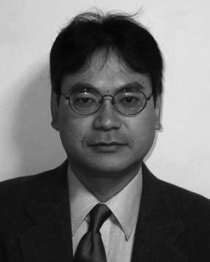 Yasushi Kanazawa合作论文数Toyohashi University of Technology50
 Hirotaka Niitsuma合作论文数Department of Computer Science, Okayama University13
 Naoya Ohta合作论文数Gunma University12Chikara Matsunaga合作论文数8
 Prasanna Rangarajan合作论文数Department of Computer Science;Department of Electrical Engineering;Department of Computer Science|Department of Electrical Engineering7
 Hanno Ackermann合作论文数Qualcomm7Atsutada Nakatsuji合作论文数6
 Ali A. Al-Sharadqah合作论文数Corresponding author.4
 Daniel Morris合作论文数Electrical and Computer Engineering, University Research Organization, Michigan State University4
 Nikolai Chernov合作论文数Department of Mathematics University of Alabam, Birmingham4Kazunari Watanabe合作论文数3
 Takeo Kanade合作论文数Robotics Institute, Carnegie Mellon University3Chika Matsunaga合作论文数3Osamu Ishikawa合作论文数2
 Anton Van Den Hengel合作论文数School of Computer Science, The University of Adelaide2
 Wojciech Chojnacki合作论文数School of Computer Science, University of Adelaide2Masatoshi Sakamoto合作论文数2Mitsuhiro Hibino合作论文数2Yasuhiro Onodera合作论文数2Yasuyuki Sugayay合作论文数2Akinobu Mori合作论文数2Tomonari Masuzaki合作论文数2
 Michael Brooks合作论文数School of Computer and Mathematical Sciences, Faculty of Sciences, Engineering and Technology, The University of Adelaide2
 Takeshi Yao (八尾健)合作论文数National Institute of Technology, Kagawa College;Kyoto University2Naoki Yano合作论文数2A Nakatuji合作论文数1A. Dick合作论文数1
 Padmanabhan Anandan合作论文数1
 Josef Bigun合作论文数School of Information Technology, Halmstad University1general chairs合作论文数1Seong-Uk Kim合作论文数1Rama Chellappa合作论文数1Hiroshi Kawasaki合作论文数1SEITARO ASAHARA合作论文数1
 Francois Bernard Lauze合作论文数Department of Computer Science, Faculty of Science, University of Copenhagen1Fabian Langguth合作论文数TU Darmstadt1Ognjen Arandjelovic合作论文数1
 Takashi Matsuyama (松山隆司)合作论文数Department of Intelligence Science and Technology, Graduate School of Informatics, Kyoto University1Yuichi Matsushita合作论文数1
 Kent Fujiwara合作论文数LY Corporation1
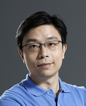 Jiaya Jia (贾佳亚)合作论文数Department of Computer Science and Engineering, The Hong Kong University of Science and Technology1
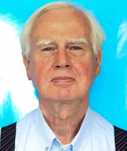 Bob Duin合作论文数Faculty of Electrical Engineering, Mathematics and Computer Science, Delft University of Technology;Faculty of Applied Sciences, Delft University of Technology1
 Hiroshi Ishikawa (石川博)合作论文数Department of Computer Science and Engineering, School of Fundamental Science and Engineering, Waseda University1
 David Suter合作论文数School of Science, Edith Cowan University1
 Martin Fuchs合作论文数Faculty of Mathematics, University of Vienna1
 Aaron Hertzmann合作论文数Computer Science and Engineering Department, Paul G. Allen School of Computer Science & Engineering, University of Washington;Adobe Systems1
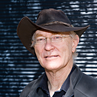 Richard Hartley合作论文数Department of Systems Engineering, Australian National University;School of Computing, Australian National University;National ICT Australia1
 Katsushi Ikeuchi合作论文数Microsoft;University of Tokyo1




