Fingertip positions can be conceptualized as Brownian particles within a force field. Using stochastic differential equations (SDEs) the force field and its associated potential function can be formally related to observed fingertip positions. Using observed fingertip positions the force field can then be “solved.” This provides a means of describing, comparing, and simulating finger-movement trajectories without formulating the kinematics of the hand. Through discretization of SDEs, the resulting mathematical forms are merely regression equations, which can be solved using familiar mathematical tools such as ordinary least squares and maximum likelihood estimation. Experimental “effects” are specified in the force-field part of the regression, and the Brownian perturbances as the random error of the regression. Using SDEs to specify potential functions can support haptic scientists performing exploratory data analysis, wishing to summarize finger-movement trajectories, compare and test differences in finger-movement trajectories between participants, groups of participants, or experimental conditions, and simulate/predict finger-movement trajectories.
Fingertip positions can be tracked using a variety of motion capture methods, raising the question of how to describe, compare, measure effects on, and simulate finger-movement trajectories. This paper provides a solution using stochastic differential equations (SDEs). In this approach, finger positions are conceptualized as Brownian particles. Effects on finger positions, from the stimulus and experimental manipulations, are formalized using a potential function and associated force field. Unlike previous SDE approaches to model animal movements, the current treatment relates fingertip positions and potential functions using SDEs that account for movement persistence. Using the SDE approach, observed fingertip positions can be used to “solve” the potential function through conventional regression methods. The resulting potential functions can be used to summarize finger-movement trajectories, and to compare and simulate trajectories.
A time series is a stretch of values on the same scale indexed by a time-like parameter. The basic data and parameters are functions. Time series take on a dazzling variety of shapes and forms, indeed there are as many time series as there are functions of real numbers.
Jerzy Neyman and Elizabeth Scott developed the idea of synthetic plots. These plots are a display of the data values of an experiment side by side with a display of simulated data values, with the simulation-based on a considered stochastic model. The Neyman and Scott work concerned the distribution of galaxies on the celestial sphere. A review of their wo is presented here followed by personal examples from hydrology, neuroscience, and animal motion.
A series of fire experiments were carried out in a wind tunnel at the United States Forest Service's Fire Science Laboratory in Missoula, Montana. The experiments involved tines cut out of pieces of cardboard. The pieces were laid out in comb‐like strips parallel to each other along a testbed. They were ignited at the windward end of the testbed. The progress of the fire was monitored by thermocouples, recording temperature, set out equidistantly up the middle of the testbed. Goals of the experiment included improved understanding of wildfire spread and the development of practical tools for wild land fire managers to employ. There was to be a search for regular pulsing in the series and any other interesting phenomena. This paper presents the results of a variety of exploratory data analyses meant to elicit information concerning the series before commencing probability modeling. Published 2014. This article is a U.S. Government work and is in the public domain in the USA.
During the 1950s the Australian entomologist Alexander Nicholson studied a sheep pest, lucilia cuprina , (L cuprina), the sheep‐blowfly. In laboratory experiments blowfly populations were set up in cages. They were supplied with necessary food and water and every other day counts were made of the numbers in their various stages of development. The experiments went on for over a year. Various statistical studies have been carried out on their data. Sadly, the bulk of the data appears to be lost. Recently this author made the discovery of total population counts for ten Nicholson experiments. These data were in a collection of copies of index cards he made during a trip to Australia in 1977. In eight of the experiments the input food was varied cyclically in sawtooth fashion, each experiment having a different period of application. However, and what is the concern of this article, which data set went with which period of application remains unclear. In the present study use is made of periodograms, spectrograms and seasonal adjustment to seek a one‐to‐one correspondence between series and period. The estimate constructed is consistent under smoothing and limiting conditions. It is time domain based, but confirmed by periodogram and spectrogram computation. Copyright © 2013 John Wiley & Sons Ltd
The paper's concern is the estimation of the average monthly temperature across a given region as a function of time. The region studied here is the Canadian province of Ontario and the time unit is month. Data for various stations and times were obtained from the Berkeley Earth website, (http://www.berkeleyearth.org). In this paper a generalized additive model with random effects is employed that allows both spatial and temporal dependence. Handling variability in both space and time is basic.
The renowned Australian entomologist Alexander J. Nicholson carried out a series of experiments in the 1950s with the intent of learning more about a sheep pest, the blowfly. The results presented here are driven by analyses of the data that Nicholson collected. The situation is of special interest because it involves a system that is nonlinear, has time lags and might be described as non‐stationary. There are other complicating aspects including that: the data are aggregate referring to a sum of interacting cohorts, age effects exist, the data are measured at discrete times yet the phenomenon exists in continuous time and a structural change may be taking place. In the work, the spectrogram and complex demodulation prove to be useful tools since the phenomenon is varying, depending on both time and period (or frequency). These tools have in common the notion of an evolutionary spectrum. The goals are to explore some of Nicholson’s data and to illustrate how the tools of complex demodulation and the spectrogram and subject matter can elicit information from time‐series data.
AbstractA spatial–temporal point process (also called space–time or spatio‐temporal point process) is a random collection of points, where each point represents the time and location of an event. Examples of events include incidence of disease, sightings or births of a species, or the occurrences of fires, earthquakes, lightning strikes, tsunamis, or volcanic eruptions. Typically the spatial locations are recorded in three spatial coordinates, e.g. longitude, latitude, and height or depth, though sometimes only one or two spatial coordinates are available or of interest.
Part 1: Theoretical Statistics.- Part 2. Time Series Papers.- Part 3. Population Biology and Environment.- Part 4. Point Processes.
DAVID HAROLD BLACKWELL, a scholar of mathematics and statistics, died of natural causes in Berkeley, California. He was a member of many communities and a role model for all.David was born at home in the small southern Illinois town of Centralia. His parents had met there. His father, Grover, was a railroad hostler, that is, the person who takes the locomotive to the roundhouse at the end of a run. David enjoyed trains his whole life and remarked, still get a special feeling every time I see a picture of a steam locomotive. His mother, Ann, was born in Mississippi. Her family moved to Centraba, where her father founded a grocery store. David learned to read from seed packets in that store. He studied at integrated public schools, completing elementary education in six years, rather than the usual eight. He has described high school as fabulous. In that period he prepared his first publication, a solution of a problem in a mathematics magazine. Of that time he remarked, really fell in love with mathematics.David's college education was all at the University of Illinois, which he entered aged sixteen. In 1938, after three years of study, he obtained an A.B. degree. An A.M. followed in 1939, and then a Ph.D. in 1941. His thesis supervisor was Joseph L. Doob, and his thesis was titled Properties of Markov Chains. Markov chains and processes became a lifelong interest of David's. Concerning his research results David would wonder, What will Joe Doob think of this? In 1966 David received a D.Sc. from that alma mater.During the period 1941-42 David held a Rosenwald Fellowship at the Institute for Advanced Study in Princeton. He experienced discrimination in Princeton; in particular, he was not allowed into Fine Hall, the mathematics building on the university campus. Two people were not allowed to enter. One was a German and the other an African American - David.In the summer of 1942 David became an assistant statistician with the Office of Price Administration in Washington, D.C. Then followed a year as instructor at Southern University in Baton Rouge. The next year he took a position as instructor at Clark College in Atlanta. David was introduced to his future wife, Ann, at Clark when he was about to teach a physics course and Ann came to register. In 1944 David went to a regular position at Howard University in D.C. Ann and he married shortly after his arrival there. He was head of the Howard mathematics department from 1947 to 1954.In 1945 he began working on statistics problems following a lecture by M. A. Girshick. He has described Girshick as his mentor in statistics. In 1954 he left Howard for what would become a lasting position at the University of California in Berkeley. In 1948-50 David spent summers at the Rand Corporation in Santa Monica. There he worked with and acknowledged the influence of K. Arrow, R. Bellman, A. Girshick, and J. Savage, amongst others. At Rand he co-authored some ten technical reports, mainly concerning military problems. There was also an article on poker strategy written with Bellman that was featured on the cover of Scientific American. He was a visiting professor of statistics at Stanford University during 1950-51.The internationally renowned statistician Jerzy Neyman came to Berkeley in 1938. In 1944 he tried to have David appointed to the mathematics department; once again, however, David experienced disabling discrimination. The then department chair's wife objected strongly. She wished not to have to entertain David at her home. To his great regret Neyman dropped the idea. However, he tried again in 1955, when a statistics department was being formed, and this time succeeded. Blackwell joined a department made up of world-renowned figures. In particular the then professors were Blackwell, Lehmann, Loeve, Neyman, and Scheffe. For many years Berkeley was considered to have the strongest statistics department in the world.David had broad interests in pure and applied mathematics. …
Abstract A temporal point process is a random process whose realizations consist of the times {τ j }, τ j ∈ ℝ, j = 0, ±1, ±2, … of isolated events scattered in time. A point process is also known as a counting process or a random scatter. The times may correspond to events of several types.
 Haiganoush K. Preisler合作论文数Pacific Southwest Research Station, Forest Service, U.S. Department Of Agriculture12
 Peter Guttorp合作论文数Department of Statistics;University of Washington;Department of Statistics, University of Washington8
 Brent Scott Stewart合作论文数7
 Luisa Fernholz合作论文数Temple University Dept. of Statistics6
 Alan Ager合作论文数Department of Forest Engineering, Resources & Management, College of Forestry, Oregon State University;Rocky Mountain Research Station, Missoula Fire Sciences Laboratory;Department of Natural Resources, Forest Research Centre, School of;Agriculture, University of Lisbon5
 Stephan Morgenthaler合作论文数4
 John G Kie合作论文数Pacific Southwest Forest;Condition of Individuals4
 Ba Bolt合作论文数3
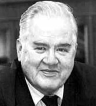 John Tukey合作论文数Princeton University3
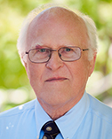 Robert M. Glaeser合作论文数University of California, Berkeley;Lawrence Berkeley National Laboratory3
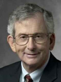 Richard A. Olshen合作论文数Department of Biomedical Data Science, School of Medicine, Stanford University3
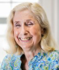 Grace Wahba合作论文数Department of Statistics, College of Letters & Science, University of Wisconsin-Madison3Jose P. Segundo合作论文数2M Hatanaka合作论文数2JR Rosenberg合作论文数2
 Rick Schoenberg合作论文数Department of Statistics, College of Physical Sciences, University of California2
 Kenneth H. Downing合作论文数Molecular Biophysics and Integrated Bioimaging Division, Lawrence Berkeley National Laboratory2
 William S. Cleveland合作论文数Department of Statistics, College of Science, Purdue University2
 Morash Valerie S合作论文数2
 Peter J. Bickel合作论文数Department of Statistics, University of California, Berkeley2
 Trevor Hastie合作论文数Department of Biomedical Data Science, School of Medicine, Stanford University;Department of Statistics, School of Humanities and Sciences, Stanford University2John W Benoit合作论文数2
 Rob Tibshirani合作论文数Department of Statistics, Stanford University;Department of Biomedical Data Science, Stanford University2
 Kerry Sieh合作论文数Geology Department, College of Science and Engineering, Western Washington University;Earth Observatory of Singapore, Nanyang Technological University;National Taiwan University2Leo Breiman合作论文数2
 Charles L. Littnan合作论文数Pacific Islands Fisheries Science Center2
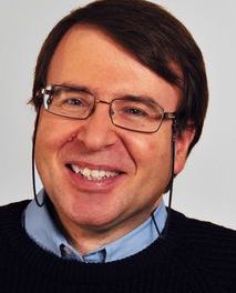 Alessandro Villa合作论文数Department of Information Systems, Faculty of Business and Economics, Université De Lausanne;Faculty of Law, Criminal Justice and Public Administration, Université De Lausanne2
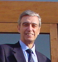 Agustín Udías Vallina合作论文数Facultad de Ciencias Físicas, Universidad Complutense de Madrid2H. D. Brunk合作论文数2D Clayton合作论文数1Carl Evans合作论文数1M. B. Priestley合作论文数1J. M. Quoniam合作论文数1Aa Georgiev合作论文数1Jm Chambers合作论文数1Dz Djokovic合作论文数1A. M. Amjad合作论文数1B. Kleiner合作论文数1Re Burgan合作论文数1Am Herzberg合作论文数1AC Atkinson合作论文数1Df Andrews合作论文数1D. J. Lewis合作论文数1Donald Taranto合作论文数1Arthur Mattuck合作论文数1F OSULLIVAN合作论文数1paul w tidwell合作论文数1P Z Marmarelis合作论文数1p r krishnaiah合作论文数1




