Summary Scientific investigation is of value only insofar as relevant results are obtained and communicated, a task that requires organizing, evaluating, analysing and unambiguously communicating the significance of data. In this context, working with ecological data, reflecting the complexities and interactions of the natural world, can be a challenge. Recent innovations for statistical analysis of multifaceted interrelated data make obtaining more accurate and meaningful results possible, but key decisions of the analyses to use, and which components to present in a scientific paper or report, may be overwhelming. We offer a 10‐step protocol to streamline analysis of data that will enhance understanding of the data, the statistical models and the results, and optimize communication with the reader with respect to both the procedure and the outcomes. The protocol takes the investigator from study design and organization of data (formulating relevant questions, visualizing data collection, data exploration, identifying dependency), through conducting analysis (presenting, fitting and validating the model) and presenting output (numerically and visually), to extending the model via simulation. Each step includes procedures to clarify aspects of the data that affect statistical analysis, as well as guidelines for written presentation. Steps are illustrated with examples using data from the literature. Following this protocol will reduce the organization, analysis and presentation of what may be an overwhelming information avalanche into sequential and, more to the point, manageable, steps. It provides guidelines for selecting optimal statistical tools to assess data relevance and significance, for choosing aspects of the analysis to include in a published report and for clearly communicating information.
Nosema ceranae is an obligate intracellular parasite and the etiologic agent of Nosemosis that affects honeybees. Beside the stress caused by this pathogen, honeybee colonies are exposed to pesticides under beekeeper intervention, such as acaricides to control Varroa mites. These compounds can accumulate at high concentrations in apicultural matrices. In this work, the effects of parasitosis/acaricide on genes involved in honeybee immunity and survival were evaluated. Nurse bees were infected with N. ceranae and/or were chronically treated with sublethal doses of coumaphos or tau-fluvalinate, the two most abundant pesticides recorded in productive hives. Our results demonstrate the following: (1) honeybee survival was not affected by any of the treatments; (2) parasite development was not altered by acaricide treatments; (3) coumaphos exposure decreased lysozyme expression; (4) N. ceranae reduced levels of vitellogenin transcripts independently of the presence of acaricides. However, combined effects among stressors on imagoes were not recorded. Sublethal doses of acaricides and their interaction with other ubiquitous parasites in colonies, extending the experimental time, are of particular interest in further research work.
In their paper, Fuller et al. (2013) compared vigilance in habitat types that differed greatly in prey abundance and proximity to cover from which predators could launch surprise attacks. Results revealed that foragers formed larger and denser flocks in habitats closer to cover. Individual vigilance of foragers in all habitats declined with increasing flock size and increased with flock density. Nevertheless, vigilance by foragers in habitats closer to cover was always higher for a given flock size than vigilance by foragers in habitats further from cover, and habitat remained an important predictor of vigilance when comparing competing models including a range of potential confounding variables. Using these data as illustration, we discuss procedures of a generalised additive mixed model (GAMM) with a Poisson distribution. The results that we obtain in our analysis are similar to those presented by Fuller and collaborators, despite the fact that they used linear mixed effects models on log-transformed data.
Chapter 1 provides a basic introduction to Bayesian statistics and Markov Chain Monte Carlo (MCMC), as we will need this for most analyses. If you are familiar with these techniques we suggest quickly skimming through it. In Chapter 2 we analyse nested zero inflated data of sibling negotiation of barn owl chicks. We explain application of a Poisson GLMM for 1-way nested data and discuss the observation-level random intercept to allow for overdispersion. We show that the data are zero inflated and introduce zero inflated GLMM. We recommend reading this chapter in detail, as we will refer often to it. Data of sandeel otolith presence in seal scat is analysed in Chapter 3. We present a flowchart of steps in selecting the appropriate technique: Poisson GLM, negative binomial GLM, Poisson or negative binomial GAM, or GLMs with zero inflated distribution. Chapter 4 is relevant for readers interested in the analysis of (zero inflated) 2-way nested data. The chapter takes us to marmot colonies: multiple colonies with multiple animals sampled repeatedly over time. Chapters 5 - 7 address GLMs with spatial correlation. Chapter 5 presents an analysis of Common Murre density data and introduces hurdle models using GAM. Random effects are used to model spatial correlation. In Chapter 6 we analyse zero inflated skate abundance recorded at approximately 250 sites along the coastal and continental shelf waters of Argentina. Chapter 7 also involves spatial correlation (parrotfish abundance) with data collected around islands, which increases the complexity of the analysis. GLMs with residual conditional auto-regressive correlation structures are used. In Chapter 8 we apply zero inflated models to click beetle data. Chapter 9 is relevant for readers interested in GAM, zero inflation, and temporal auto-correlation. We analyse a time series of zero inflated whale strandings. In Chapter 10 we demonstrate that an excessive number of zeros does not necessarily mean zero inflation. We also discuss whether the application of mixture models requires that the data include false zeros and whether the algorithm can indicate which zeros are false.
Chapter 9 Estimation of Common Trends for Trophic Index Series Alain F. Zuur, Alain F. Zuur Highland Statistics Ltd, 6 Laverock Road, Newburgh AB41 6FN, UKSearch for more papers by this authorElena N. Ieno, Elena N. Ieno Highland Statistics, Suite N 226, Av Finlandia 21, CC Gran Alacant Local 9, 03130 Santa Pola, SpainSearch for more papers by this authorCristina Mazziotti, Cristina Mazziotti ARPA Emilia-Romagna, Struttura Oceanografica Daphne, V le Vespucci 2, 47042 Cesenatico (FC), ItalySearch for more papers by this authorGiuseppe Montanari, Giuseppe Montanari ARPA Emilia-Romagna, Struttura Oceanografica Daphne, V le Vespucci 2, 47042 Cesenatico (FC), ItalySearch for more papers by this authorAttilio Rinaldi, Attilio Rinaldi ARPA Emilia-Romagna, Struttura Oceanografica Daphne, V le Vespucci 2, 47042 Cesenatico (FC), ItalySearch for more papers by this authorCarla Rita Ferrari, Carla Rita Ferrari ARPA Emilia-Romagna, Struttura Oceanografica Daphne, V le Vespucci 2, 47042 Cesenatico (FC), ItalySearch for more papers by this author Alain F. Zuur, Alain F. Zuur Highland Statistics Ltd, 6 Laverock Road, Newburgh AB41 6FN, UKSearch for more papers by this authorElena N. Ieno, Elena N. Ieno Highland Statistics, Suite N 226, Av Finlandia 21, CC Gran Alacant Local 9, 03130 Santa Pola, SpainSearch for more papers by this authorCristina Mazziotti, Cristina Mazziotti ARPA Emilia-Romagna, Struttura Oceanografica Daphne, V le Vespucci 2, 47042 Cesenatico (FC), ItalySearch for more papers by this authorGiuseppe Montanari, Giuseppe Montanari ARPA Emilia-Romagna, Struttura Oceanografica Daphne, V le Vespucci 2, 47042 Cesenatico (FC), ItalySearch for more papers by this authorAttilio Rinaldi, Attilio Rinaldi ARPA Emilia-Romagna, Struttura Oceanografica Daphne, V le Vespucci 2, 47042 Cesenatico (FC), ItalySearch for more papers by this authorCarla Rita Ferrari, Carla Rita Ferrari ARPA Emilia-Romagna, Struttura Oceanografica Daphne, V le Vespucci 2, 47042 Cesenatico (FC), ItalySearch for more papers by this author Book Editor(s):Richard E. Chandler, Richard E. Chandler Department of Statistical Science, UCL, Gower Street, London WC1E 6BT, UKSearch for more papers by this authorE. Marian Scott, E. Marian Scott School of Mathematics and Statistics, University of Glasgow, Glasgow G12 8QW, UKSearch for more papers by this author First published: 18 March 2011 https://doi.org/10.1002/9781119991571.ch9 AboutPDFPDF ToolsRequest permissionExport citationAdd to favoritesTrack citation ShareShareShare a linkShare onEmailFacebookTwitterLinkedInRedditWechat Summary This chapter discusses the multimetric TRophic IndeX (TRIX). It describes the effects of pollution over time, in order to inform management strategies such as cleanup operations and to set new regulations. The chapter presents two different statistical approaches. First it uses additive models incorporating temporal autocorrelation along with a spatial residual correlation structures. In the second approach, dynamic factor analysis (DFA) is used. The chapter can be regarded as a guide to the model-building process for practitioners. It also discusses a univariate smoothing method to estimate underlying patterns in multivariate time series. The chapter uses additive modelling, taking a step-by-step approach to the development of an appropriate model for the TRIX series. It considers two rather different modelling approaches to investigate trends in eutrophication, as measured using TRIX, along the coast of the Emilia-Romagna region. Controlled Vocabulary Terms autocorrelation; factor analysis; multivariate time series analysis; trend References Barbour, M. T., Stribling, J. B. and Karr, J. (1995) Multimetric approach for establishing biocriteria and measuring biological conditions. In Biological Assessment and Criteria – Tools for Water Resources Planning and Decision Making (eds. W. S. Davis and T. P. Simon). Lewis Publishers, Boca Raton, Florida. pp. 63–77. Web of Science®Google Scholar Bowman, A., Giannitrapani, M. and Scott, E. M. (2009) Spatiotemporal smoothing and sulphur dioxide trends over Europe. Journal of the Royal Statistical Society, Series C, 58, 737–752. 10.1111/j.1467-9876.2009.00671.x Web of Science®Google Scholar Chen, C. S., Pierce, G. J., Wang, J., Robin, J. P., Poulard, J. C., Pereira, J., Zuur, A. F., Boyle, P. R., Bailey, N., Beare, D. J., Jereb, P., Ragonese, S., Mannini, A. and Orsi-Relini, L. (2006) The apparent disappearance of Loligo forbesi from the south of its range in the 1990s: trends in Loligo spp. abundance in the northeast Atlantic and possible environmental influences. Fisheries Research, 78, 44–54. 10.1016/j.fishres.2005.12.002 Web of Science®Google Scholar de Wit, M. and Bendoricchio, G. (2001) Nutrient fluxes in the Po basin. Science of the Total Environment, 273, 147–161. 10.1016/S0048-9697(00)00851-2 CASPubMedWeb of Science®Google Scholar Diaz, R., Solan, M. and Valente, R. (2004) A review of approaches for classifying benthic habitats and evaluating habitat quality. Journal of Environmental Management, 73, 165–181. 10.1016/j.jenvman.2004.06.004 PubMedWeb of Science®Google Scholar Draper, N. R. and Smith, H. (1998) Applied Regression Analysis, 3rd edition. John Wiley and Sons, Inc., New York. 10.1002/9781118625590 Google Scholar Erzini, K. (2005) Trends in NE Atlantic landings (southern Portugal): identifying the relative importance of fisheries and environmental variables. Fishing and Oceanography, 14, 195–209. 10.1111/j.1365-2419.2005.00332.x Web of Science®Google Scholar Erzini, K., Inejih, C. and Stobberup, K. A. (2005) An application of two techniques for the analysis of short, multivariate non-stationary time series of Mauritanian trawl survey data. ICES Journal of Marine Science, 62, 353–359. 10.1016/j.icesjms.2004.12.009 Web of Science®Google Scholar Everitt, B. S. and Dunn, G. (2001) Applied Multivariate Data Analysis, 2nd edition. Arnold, London. 10.1002/9781118887486 Google Scholar Faraway, J. J. (2005) Extending the Linear Model with R: Generalized Linear, Mixed Effects and Nonparametric Regression Models. Chapman & Hall/CRC, Boca Raton, Florida. 10.1201/b15416 Google Scholar Fausch, K. D., Lyons, J., Karr, J. R. and Angermeier, P. L. (1990) Fish communities as indicators of environmental degradation. American Society Symposium, 8, 123–144. Google Scholar Fitzmaurice, G. M., Laird, N. M. and Ware, J. H. (2004) Applied Longitudinal Analysis. John Wiley & Sons, Inc., Hoboken, New Jersey. 10.1198/jasa.2009.0116 CASWeb of Science®Google Scholar Fletcher, R. L. (1996) The occurrence of green tides – a review. In Marine Benthic Vegetation: Recent Changes and the Effects of Eutrophication (eds. W. Schramm and P. H. Neinhuis). Springer, New York. pp. 7–44. 10.1007/978-3-642-61398-2_2 Web of Science®Google Scholar Giovanardi, F. and Vollenweider, R. A. (2004) Trophic conditions of marine coastal waters: experience in applying the trophic index TRIX to two areas of the Adriatic and Tyrrhenian seas. Journal of Limnology, 63(2), 199–218. 10.4081/jlimnol.2004.199 Google Scholar Harvey, A. C. (1989) Forecasting, Structural Time Series Models and the Kalman Filter. Cambridge University Press, Cambridge. Google Scholar Hastie, T. and Tibshirani, R. (1990) Generalized Additive Models. Chapman & Hall, London. Web of Science®Google Scholar Laine, A. O., Andersin, A. B., Leiniö, S. and Zuur, A. F. (2006) Stratification induced hypoxia as a structuring factor of macrozoobenthos in the open Gulf of Finland (Baltic Sea). Journal of Sea Research. Google Scholar Mendelssohn, R. and Schwing, F. B. (2002) Common and uncommon trends in SST and wind stress in the California and Peru–Chile current systems. Progress in Oceanography, 53(2–4), 141–162. 10.1016/S0079-6611(02)00028-9 Web of Science®Google Scholar Molenaar, P. C. M. (1985) A dynamic factor model for the analysis of multivariate time series. Psychometrika, 50, 181–202. 10.1007/BF02294246 Web of Science®Google Scholar Montgomery, D. C. and Peck, E. (1992) Introduction to Linear Regression Analysis. John Wiley & Sons, Inc., New York. Google Scholar Pinheiro, J. C. and Bates, D. M. (2000) Mixed-Effects Models in S and S-PLUS. Springer-Verlag, New York. 10.1007/978-1-4419-0318-1 PubMedWeb of Science®Google Scholar Pinheiro, J. C., Bates, D. M., DebRoy, S. and Sarkar, D. (2008) nlme: Linear and Nonlinear Mixed Effects Models. R package version 3.1-89. Google Scholar Pompei, M., Ghetti, A., Milandri, A. and Mazziotti, C. (1995) Fioriture microalgali ed evoluzione dei principali popolamenti fitoplanctonici nelle acque costiere Emiliano-Romagnole dal 1982 al 1994. In Proceedings of Conference 'Evoluzione dello stato trofico in Adriatico analisi di interventi attuati e future linee di intervento', pp. 51–60, Marina di Ravenna, Italy, September. Google Scholar Quinn, G. P. and Keough, M. J. (2002) Experimental Design and Data Analysis for Biologists. Cambridge University Press, Cambridge. 10.1017/CBO9780511806384 Google Scholar Rinaldi, A. and Montanari, G. (1988) Eutrophication in Emilia-Romagna coastal waters in 1984– 1985. Annals of New York Academy of Science, 534, 959–977. 10.1111/j.1749-6632.1988.tb30188.x CASWeb of Science®Google Scholar Shumway, R. H. and Stoffer, D. S. (1982) An approach to time series smoothing and forecasting using the EM algorithm. Journal of Time Series Analysis, 3, 253–264. 10.1111/j.1467-9892.1982.tb00349.x Google Scholar Shumway, R. H. and Stoffer, D. S. (2000) Time Series Analysis and Its Applications. Springer-Verlag, New York. 10.1007/978-1-4757-3261-0 Google Scholar Vollenweider, R. A. (1968) Scientific fundamentals of eutrophication of lakes and flowing waters, with particular reference to nitrogen and phosphorus as factors in eutrophication. Technical Report, DAS/CSI/68.27., OECD, Paris. Google Scholar Vollenweider, R. A. (1981) Eutrophication a global problem. WHO Water Quality Bulletin, 6(3), 59–62. Google Scholar Vollenweider, R. A., Montanari, F. G. G. and Rinaldi, A. (1998) Characterization of the trophic conditions of marine coastal waters, with special reference to the NW Adriatic Sea: proposal for a trophic scale, turbidity and generalized water quality index. Environmetrics, 9, 329–357. 10.1002/(SICI)1099-095X(199805/06)9:3<329::AID-ENV308>3.0.CO;2-9 CASWeb of Science®Google Scholar Vollenweider, R. A., Rinaldi, A. and Montanari, G. (1992) Eutrophication, structure and dynamics of a marine coastal system: results of 10-year monitoring along the Emilia-Romagna coast (northwest Adriatic Sea). In Science of the Total Environment, Supplement 1992 – Marine Coastal Eutrophication (eds. R. A. Vollenweider, R. Marchetti and R. Viviani), pp. 63–106. Web of Science®Google Scholar Webster, R. and Oliver, M. A. (2001) Geostatistics for Environmental Scientists. John Wiley & Sons, Ltd, Chichester. Google Scholar Wood, S. N. (2006) Generalized Additive Models: An Introduction with R. Chapman & Hall/CRC, Boca Raton, Florida. 10.1201/9781420010404 Google Scholar Zuur, A. F., Ieno, E. N. and Elphick, C. S. (2010) A protocol for data exploration to avoid common statistical problems. Methods in Ecology and Evolution, 1(1), 3–14. 10.1111/j.2041-210X.2009.00001.x Web of Science®Google Scholar Zuur, A. F., Ieno, E. N. and Smith, G. M. (2007) The Analysis of Ecological Data. Springer-Verlag, New York. 700 pp. Google Scholar Zuur, A. F. and Pierce, G. J. (2004) Common trends in northeast Atlantic squid time series. Journal of Sea Research, 52, 57–72. 10.1016/j.seares.2003.08.008 Web of Science®Google Scholar Zuur, A. F., Tuck, I. D. and Bailey, N. (2003) Dynamic factor analysis to estimate common trends in fisheries time series. Canadian Journal of Fisheries and Aquatic Sciences, 60, 542–552. 10.1139/f03-030 Web of Science®Google Scholar Zuur, A. F., Fryer, R. J., Jolliffe, I. T., Dekker, R. and Beukema, J. J. (2003) Estimating common trends in multivariate time series using dynamic factor analysis. Environmetrics, 14(7), 665–685. 10.1002/env.611 Web of Science®Google Scholar Zuur, A. F., Ieno, E. N., Walker, N., Saveliev, A. A. and Smith, G. M. (2009) Mixed Effects Models and Extensions in Ecology with R. Springer-Verlag, New York. xxii + 574 pp. 10.1007/978-0-387-87458-6 Google Scholar Statistical Methods for Trend Detection and Analysis in the Environmental Sciences ReferencesRelatedInformation
We analyzed long-term winter survey data (1956–2007) for three endangered waterbirds endemic to the Hawaiian Islands, the Hawaiian moorhen ( Gallinula chloropus sandvicensis ), Hawaiian coot ( Fulica alai ), and Hawaiian stilt ( Himantopus mexicanus knudseni ). Time series were analyzed by species–island combinations using generalized additive models, with alternative models compared using Akaike information criterion (AIC). The best model included three smoothers, one for each species. Our analyses show that all three of the endangered Hawaiian waterbirds have increased in population size over the past three decades. The Hawaiian moorhen increase has been slower in more recent years than earlier in the survey period, but Hawaiian coot and stilt numbers still exhibit steep increases. The patterns of population size increase also varied by island, although this effect was less influential than that between species. In contrast to earlier studies, we found no evidence that rainfall affects counts of the target species. Significant population increases were found on islands where most wetland protection has occurred (Oahu, Kauai), while weak or no increases were found on islands with few wetlands or less protection (Hawaii, Maui). Increased protection and management, especially on Maui where potential is greatest, would likely result in continued population gains, increasing the potential for meeting population recovery goals.
1. While teaching statistics to ecologists, the lead authors of this paper have noticed common statistical problems. If a randomsample of their work (including scientific papers) produced before doing these courses were selected, half would probably contain violations of the underlying assumptions of the statistical techniques employed.2. Some violations have little impact on the results or ecological conclusions; yet others increase type I or type II errors, potentially resulting in wrong ecological conclusions. Most of these violations can be avoided by applying better data exploration. These problems are especially troublesome in applied ecology, where management and policy decisions are often at stake.3. Here, we provide a protocol for data exploration; discuss current tools to detect outliers, heterogeneity of variance, collinearity, dependence of observations, problems with interactions, double zeros in multivariate analysis, zero inflation in generalized linear modelling, and the correct type of relationships between dependent and independent variables; and provide advice on how to address these problems when they arise. We also address misconceptions about normality, and provide advice on data transformations.4. Data exploration avoids type I and type II errors, among other problems, thereby reducing the chance of making wrong ecological conclusions and poor recommendations. It is therefore essential for good quality management and policy based on statistical analyses.
Forensic pathologists and entomologists estimate the minimum post-mortem interval since a long time by describing the stage of succession and development of the necrophagous fauna (Amendt et al. 2004). From very simple calculations at the beginning, (Bergeret, see also Smith 1986) the discipline has evolved into a more mathematical one (e.g. Marchenko 2001; Grassberger and Reiter 2001, 2002) and tries to implement concepts like probabilities and confidence intervals (Lamotte and Wells 2000; Donovan et al. 2006; Tarone and Foran 2008, see also Villet et al. this book Chapter7). As pointed out by Tarone and Foran (2008) and Van Laerhoven (2008), the latter is one of the major tenets of the Daubert Standard (Daubert et al. v. Merrell Dow Pharmaceuticals (509 U.S. 579 (1993)).
In this chapter, we discuss models for zero-truncated and zero-inflated count data. Zero truncated means the response variable cannot have a value of 0. A typical example from the medical literature is the duration patients are in hospital. For ecological data, think of response variables like the time a whale is at the surface before re-submerging, counts of fin rays on fish (e.g. used for stock identification), dolphin group size, age of an animal in years or months, or the number of days that carcasses of road-killed animals (amphibians, owls, birds, snakes, carnivores, small mammals, etc.) remain on the road. These are all examples for which the response variable cannot take a value of 0.
Datasets are frequently given as Excel worksheets. We must transfer them from Excel to R in order to place the variable names on the Rcmdr menu items. We show how to do the transfer for several different data structures. Sometimes datasets are given as ASCII text files. These too can be read into Excel and then transferred to R. Sometimes datasets are already in R. We can work with them directly, and we can display them in Excel by transferring the data the other direction from R to Excel.
In this chapter, we analyse three data sets; California birds, owls, and deer. In the first data set, the response variable is the number of birds measured repeatedly over time at two-weekly intervals at the same locations. In the owl data set (Chapter 5), the response variable is the number of calls made by all offspring in the absence of the parent. We have multiple observations from the same nest, and 27 nests were sampled. In the deer data, the response variable is the presence or absence of parasites in a deer; the data are from multiple farms.
In this chapter, we continue with Gaussian linear and additive mixed modelling methods and discuss their application on nested data. Nested data is also referred to as hierarchical data or multilevel data in other scientific fields (Snijders and Boskers, 1999; Raudenbush and Bryk, 2002).
In the previous chapter, count data with no upper limit were analysed using Poisson generalised linear modelling (GLM) and negative binomial GLM. In Section 10.2 of this chapter, we discuss GLMs for 0−1 data, also called absence–presence or binary data, and in Section 10.3 GLM for proportional data are presented. In the final section, generalised additive modelling (GAM) for these types of data is introduced. A GLM for 0−1 data, or proportional data, is also called logistic regression.
This chapter explains how correlation structures can be added to the linear regression and additive model. The mixed effects models from Chapters 4 and 5 can also be extended with a temporal correlation structure. The title of this chapter contains ‘Part I’, suggesting that there is also a Part II. Indeed, that is the next chapter. In part I, we use regularly spaced time series, whereas in the next chapter, irregular spaced time series, spatial data, and data along an age gradient are analysed. We use a bird time series data set previously analysed in Reed et al. (2007). In the first section, we start with only one species and show how the linear regression model can be extended with a residual temporal correlation structure. In the second section, we use the same approach for a multivariate time series. In Section 6.3, the owl data are used again.
A generalised linear model (GLM) or a generalised additive model (GAM) consists of three steps: (i) the distribution of the response variable, (ii) the specification of the systematic component in terms of explanatory variables, and (iii) the link between the mean of the response variable and the systematic part. In Chapter 8, we discussed several different distributions for the response variable: Normal, Poisson, negative binomial, geometric, gamma, Bernoulli, and binomial distributions. One of these distributions can be used for the first step mentioned above. In fact, later in Chapter 11, we see how you can also use a mixture of two distributions for the response variable; but in this chapter, we only work with one distribution at a time.
 Alain Zuur合作论文数Highland Statistics Ltd65
 Graham M. Smith合作论文数48
 Anatoliy A Saveliev合作论文数Kazan State University15Neil J. Walker合作论文数11
 Erik H. Meesters合作论文数Institute of Taxonomic Zoology;Institute for Sea Research;Institute of Taxonomic Zoology, Institute for Sea Research10
 Graham J. Pierce合作论文数Instituto de Investigaciones Marinas, Consejo Superior de Investigaciones Cientificas3Chris S. Elphick合作论文数2
 M. Begona Santos合作论文数Department of Zoology;University of Aberdeen;Department of Zoology, University of Aberdeen2a edridge合作论文数1
 Martin Solan合作论文数National Oceanography Centre Southampton, University of Southampton1
 Richard Fuller合作论文数School of the Environment, Faculty of Science, The University of Queensland1
 Belen Branchiccela合作论文数1
 Martin Javier Eguaras合作论文数Departamento de Biología, National University of Mar del Plata;Consejo Nacional de Investigaciones Cientificas y Tecnicas1
 Porrini Martín P合作论文数Arthropods Laboratory FCEyN, UNMdP1
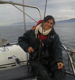 Patricia Lastra Luque合作论文数Santander Oceanographic Centre, Spanish Institute of Oceanography1Garrido Paula Melisa合作论文数1Fremdt Heike合作论文数1
 Paul M. Thompson合作论文数Imaging Genetics Center, Lab of Neuro Imaging, Institute for Neuroimaging and Informatics, Keck School of Medicine, University of Southern California1Giuseppe Montanari合作论文数1Carla Rita Ferrari合作论文数1Paul Batty合作论文数1
 Pablo Zunino合作论文数Laboratorio de Microbiología, Instituto de Investigaciones Biológicas Clemente Estable1
 Jens Amendt合作论文数Department of Medicine, Institute of Legal Medicine, Goethe University Frankfurt1
 Jennifer A Learmonth合作论文数School of Biological Sciences (Zoology),, University of Aberdeen1
 Karina Antunez合作论文数Departamento de Microbiología, Instituto de Investigaciones Biológicas Clemente Estable1
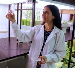 Giselle M A Martinez-Noel合作论文数1
 J. Michael Reed (Michael Reed)合作论文数Department of Biology, School of Arts and Sciences, Tufts University1
 Graciela L Salerno合作论文数Fundación para Investigaciones Biológicas Aplicadas (FIBA), Centro de Investigaciones Biológicas C.C.1
 T. (Theunis) Piersma合作论文数Faculty of Science and Engineering, University of Groningen;Groningen Institute for Evolutionary Life Sciences, University of Groningen;Centre for Ecological and Evolutionary Studies, Faculty of Mathematics and Natural Sciences, University of Groningen1Cristina Mazziotti合作论文数1




