A variety of time series signal extraction or equivalently, optimal smoothing problems are considered from a “smoothness priors” point of view. The origin of the subject is a smoothing problem posed by Whittaker (1923). Smoothness priors is treated here from a stochastic regression-linear model-Gaussian disturbances framework. This conceptually simple framework has broad applications in time series analysis. A reproducing kernel Hilbert space, (RKHS), framework illustrates some facets of smoothness priors. Power spectral density estimation and transfer function estimation for stationary time series and also the modeling of nonstationary mean and both scalar and multichannel nonstationary covariance times series are shown from a smoothness priors approach.
In this chapter we review some of the applications of smoothness priors modeling of time series that can be done by least squares, or equivalently as linear Gaussian modeling. Smoothness priors trend estimation for scalar time series is treated in Section 4.1. There, the smoothness priors constraint is expressed as a k-th order random walk with a normally distributed zero-mean, unknown variance perturbation. The (normalized) variance is a hyperparameter of the prior distribution. This constraint is a time domain constraint on the priors. The concept of frequency domain priors is introduced and exploited in Sections 4.2 and 4.3. There, the fitting of a smoothness priors long AR model for the spectrum estimation of a scalar stationary time series and a smoothness priors model for transfer function estimation between two simultaneously observed time series, are respectively shown. In addition in Section 4.2, the superiority of the smoothness priors long AR model as compared to ordinary AIC AR model order determined spectral analysis, is demonstrated by a Monte Carlo computation of entropy.
Linear Gaussian state space modeling is treated in this chapter. The prediction, filtering and smoothing formulas in the standard Kalman filter are shown. Model identification or, computation of the likelihood of the model is also treated. Some of the well known state space models that are used in this book as well as state space modeling of missing observations and a state space model for unequally spaced time series are shown. The final section is a discussion of the information square root filter/smoother, that we use in linear Gaussian state space seasonal decomposition modeling in Chapter 9. Not necessarily linear - not necessarily Gaussian state space modeling is treated in Chapter 6. A variety of illustrative examples of linear state space modeling is shown in Chapter 7.
The early development of time series has been related to a quest for an understanding of cyclical phenomena. For example, Shuster’s periodogram (1898, 1906), and Yule’s (1927) introduction of autoregressive models, were devoted to the analysis of cyclical sunspot numbers and Whittle’s (1954) analysis of the water level in a rock channel on the Wellington coast of New Zealand is also related to a cyclical phenomenon. In fact many time series exhibit cyclical behavior in the sense there appears to be an approximate repetition of a pattern with a not very well defined period or amplitude. Rather both the period and amplitude appear to change gradually. Typically ecological data, air pollution data and several other physical phenomena exhibit such behavior. Two of the most familiar examples of time series which exhibit such behavior and which have been extensively analyzed are the Canadian lynx data, (for example see Campbell and Walker 1977, Tong 1977, Bhansali 1979 and Priestly 1981), and the Wolfer sunspot series, (Morris 1977, Tong 1983). Such series are frequently modeled by AR, ARMA or AR plus sinusoidal models. However, none of these modeling methods are very satisfactory for the prediction of more than one lead time, (Tong 1982). As pointed out in Akaike (1977b) in his discussion of several analyses of the Canadian lynx data, those analyses were unconvincing and that the critical issue in modeling time series is the selection of a proper model.
In this chapter we illustrate the application of non-Gaussian modeling method to the analysis of inhomogeneous discrete random processes data. Two data analytic examples, Tokyo rainfall data, a nonstationary binary process and the analysis of a simulated nonstationary Poisson process data set are shown. The latter simulation is based on research of the count of X-rays from the star Cygnus Xl data. Kashiwagi and Yanagimoto (1992), is an application of the non-Gaussian state space methodology in the analysis of nonstationary Poisson process analysis of medical data.
There are many time series whose structure involves a substantial change of variance. The decomposition of the seismic time series problem in Chapter 7 is such an example. In other practical data situations, the relatively fast wiggles of a nonstationary covariance time series appears to be modulated by a relatively slowly changing envelope function. For example, seismic measurements during an earthquake exhibit this behavior. That envelope function can be interpreted as a change of scale associated with the instantaneous innovations variance of the state space model of the time series. In this chapter the changing variance structure of the Urakawa-Oki, Hokkaido Japan March 21 1983, earthquake data, (code name MYN2F, Takanami 1991) is estimated by both Gaussian and non-Gaussian state space models. Additional applications include the change of variance modeling in the estimation of the log-periodogram of a time series and the estimation of the instantaneous variance of the collection of 21 years of daily maximum temperatures in Tokyo.
The modeling of multivariate nonstationary covariance time series is relevant to many econometric, human electroencephalogram, oceanographic, meteorological and seismic data situations. (See for example Brillinger and Hatanaka 1969, 1970.) In this chapter multivariate nonstationary covariance time series are modeled using time varying multivariate autoregressive or equivalently, time varying vector autoregressive, (TVVAR), models. This model is a natural extension of the scalar TVAR model shown in Chapter 11. Analogous to Chapter 11, two different modeling methods are presented. In one method, smoothness priors constraints are placed directly on the evolution of the individual AR parameters of the TVVAR model. In the other method, smoothness priors constraints are placed on the evolution of the PARCORs of AR models. The key idea which permits TVVAR modeling is a “one channel at-atime” paradigm. This idea is a consequence of an instantaneous response-orthogonal innovations representation of multivariate AR models. That permits the multivariate time series to be modeled one scalar AR model at-a-time.
A nonlinear state space approach to the smoothing of time series is developed. The time series is expressed in state space model form where the system model or the observation model contains nonlinear functions of the state vector. Recursive formulas for prediction, filtering and smoothing for the nonlinear state space model are shown. The performance of the method is illustrated by the analyses of both a one dimensional and a two dimensional example that have been previously considered in the literature. These examples require numerical approximations of the relevant densities and numerical computations for the nonlinear transformations of variables, the convolution of two densities, Bayes formula, and normalization. Results for the one dimensional example are compared and contrasted with those obtained by the extended Kalman filter method, by a second moment approximation method and also by the Monte Carlo filter method. An empirical study of the numerical accuracy is also shown. A more complete treatment of this material is in Kitagawa (1991).
In this chapter the ideas that we identify as the basis of our approach to time series analysis are outlined. Several topics in parameter estimation and model selection are treated. Akaike’s AIC for parametric model selection is treated first. That treatment includes a discussion of the Kullback-Leibler information, and a theoretical development of the AIC. Also included are treatments of the Householder transformation based least squares estimation, the maximum likelihood method of parameter estimation, (including a method of minimizing a function of several variables), a fairly general discussion of state space modeling including Kalman filter for standard linear Gaussian state space modeling, and general state space modeling.
The “history” of smoothness priors essentially starts with a problem addressed in Whittaker (1923). It was followed by Shiller (1973), and Akaike (1980a) in which the framework initiated by Shiller was continued Akaike (1980a) was a quasi-Bayesian Gaussian disturbances linear regression, least squares computations, model framework. Stochastic difference equation constraints were placed on the prior distributions of the model parameters. The critical computation was that of the likelihood of hyperparameters of those distributions. Our own work and a considerable amount of other work was motivated by Akaike (1980a). Here we identify some of that work and some relationship of that work to other research as well as developments and extensions. The least squares computational framework of smoothness priors is also presented here.
Some applications of the state space models that were described in Chapter 5 are presented in this chapter. In particular, the modeling of the famous Canadian lynx data by an AR state space model, the modeling of irregularly spaced data and an example of the decomposition of an observed time series into a signal, background noise and observation noise are shown.
In this chapter scalar nonstationary covariance time series are modeled using time varying coefficient autoregressive models, as in equation 11.1. In such a model for N observations, if the order of the AR model is m there will be N × m AR coefficient parameters and as many asNinnovations variance parameters. Fitting a time varying AR, (TVAR), model with smoothness priors constraints permits those parameters to be estimated implicitly in terms of only a small number of explicitly estimated hyperparameters. Several different mechanisms for implementing the smoothness priors constraints are possible. Our own approach to this important topic has evolved over several years, and two different methods for fitting the time varying AR coefficient model with smoothness priors constraints are shown here. (Each of the methods has implications for the modeling of multivariate nonstationary covariance data. That topic is treated in Chapter 12.) Our primary application for the scalar nonstationary covariance modeling is the evolution with time of the power spectrum. The estimated TVAR model yields what we refer to as an “instantaneous power spectral density”.
Non-Gaussian state space modeling of time series and the more general, general state space modeling are treated in this chapter. They were introduced because of the need to model time series with abrupt discontinuities, and time series with outliers and to model time series whose state and or observation processes were nonlinear. The general state space model and its recursive formulas for prediction, filtering and smoothing are treated in Section 6.2 after an introduction in Section 6.1. Three alternative computational approaches for realizing the general state space modeling, numerical integration method, a Gaussian mixture-two filter formula method and the most recently developed Monte Carlo “particle-path tracing” method are discussed respectively in Sections 6.3, 6.4 and 6.5. In addition, starting from the general state space model, an alternative derivation of the Kalman filter is shown in Section 6.6. Applications of the non-Gaussian methods appear in Chapters 8 through 16. In those chapters where appropriate, the non-Gaussian and general state space methods performance are contrasted with the linear Gaussian state space analysis methods.
In this paper the informational approach to statistics based on an informational interpretation of log likelihood of a statistical model is contrasted with the conventional Fisherian framework. It is pointed out that for the recognition of practical importance of statistical science more emphasis should be placed on the development of new models than the refinement of mathematical analysis of existing procedures, although the latter activity should never be ignored. This is based on the observation that it is the contribution of statistics to the development of new hypotheses for the interpretation of data that creates the importance of the subject. It is argued that the informational approach prepares a basis for the rapid expansion of the area of application of statistics by providing a theoretical foundation for the development and evaluation of new statistical models in diverse fields.
Multibeam bathymetric data is modeled from a Bayesian “smoothness priors” framework. Smoothness priors is a penalized likelihood‐nonparametric linear regression form of modeling and the bathymetry data are modeled one beam at‐a‐time. The method is applied to data previously analyzed in Goff and Jordan (1988) and Gilbert and Malinverno (1988). The results contrast nonparametric and parametric modeling, dispute the almost conventional removal of “deterministic” components prior to stochastic modeling and reveal new evidence about mid‐ocean ridge spreading processes.
A smoothness priors approach to transfer function estimation from a stationary time series is shown. An infinite order impulse response model plus an infinite order additive AR noise model is assumed. This is algebraically equivalent to an infinite order ARMAX plus white noise model. A finite order ARMAX model approximation to this model is actually fitted to data. Frequency domain smoothness priors are assumed on the ARMAX polynomials and smoothness hyperparameters balance the tradeoff between the infidelity of the model to the data and the infidelity of the model to the smoothness constraints. The likelihood of the hyperparameters is maximized by a least squares gradient search computational procedure. The method is illustrated by the analysis of the Box-Jenkins (BJ) series J data.
A unified nearest neighbor-time series analysis approach to the problem of the classification of faults in rotating machinery is developed. The procedure has an optimum minimum probability of misclassification property for normally distributed time series and near optimum misclassification properties otherwise. Examples of the classification of acceleration, pressure, and torque sensor data from stationary, locally stationary, and covariance stationary time series with mean value time functions are considered. Estimates of the probability of misclassification are computed for each situation. The underlying assumptions and properties of the nearest neighbor time series classification procedure and signature analysis procedures are compared.
 Genshiro Kitagawa (北川源四郎)合作论文数Meiji University;The Graduate University for Advanced Studies18
 tom brotherton合作论文数3A. M. Shurygin合作论文数1David Stone合作论文数1achilles g koyiantis合作论文数1
 Demetrios Kazakos合作论文数Texas Southern University1
 Tomoyuki Higuchi (樋口知之)合作论文数Institute of Statistical Mathematics;Department of Data Science for Business Innovation, Faculty of Science and Engineering, Chuo University1
 P. Papantoni-Kazakos合作论文数1Yosi Ogata合作论文数Institute of Statistical Mathematics;Graduate University for Advanced Studies1
 Masami Hasegawa合作论文数Institute of Statistical Mathematics;School of Life Sciences, Fudan University1
 Kohei Ohtsu合作论文数1Eugene Dong合作论文数1Masaharu Tanemura合作论文数1
 Dimitris A. Pados合作论文数College of Electrical Engineering and Computer Science, Florida Atlantic University1Simon G Braun合作论文数1
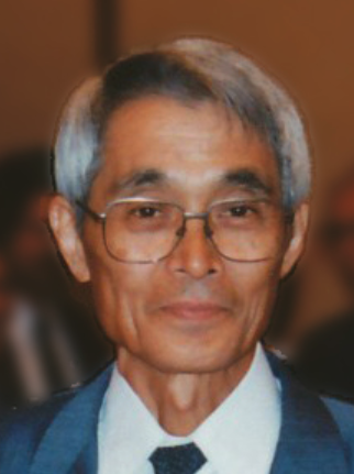 Hirotugu Akaike (赤池弘次)合作论文数The Institute of Statistical Mathematics;The Graduate University for Advance Study1David Vere-Jones合作论文数1
 Emanuel Parzen合作论文数Department of Statistics;Texas A&M University1Brotherton, T.合作论文数1




