Upper-ocean mixing regulates the vertical transport of heat, momentum, and tracers in the ocean surface boundary layer. Langmuir turbulence (LT), generated by the interaction of wind stress and wave-induced Stokes drift, is a dominant mixing mechanism in the open ocean. Observations of LT in leads, polynyas, and the marginal ice zone (MIZ) confirm its presence in ice-covered regions, but its Arctic-wide occurrence and modulation by sea ice and waves remain limited in characterization. Here we present the first pan-Arctic assessment of LT mixing potential using a coupled sea ice–wave model integrating neXtSIM and WAVEWATCH III. Using wind–wave forcing metrics, we show that LT-relevant forcing beneath sea ice is spatially confined and highly intermittent. Conditions favorable for LT largely occur within the seasonal MIZ and arise episodically. Sea ice concentration sets the mean balance between wave- and shear-driven turbulence, but does not uniquely determine LT variability. The realization of wave-driven mixing depends on wave conditions and ice structure, while wind–wave misalignment plays a secondary role. As a result, LT in the Arctic MIZ typically occurs within mixed-forcing regimes, where wave-driven and shear-driven processes coexist. Our findings highlight the importance of wave–ice interactions and intermittency in shaping upper-ocean mixing under partial ice cover.
Surface waves are becoming more prevalent in the Arctic as sea ice cover reduces. Here we use 3D turbulence-resolving simulations to explore how surface waves affect upper ocean dynamics, and hence surface conditions, as they propagate along summertime leads (narrow regions of open ocean between melting sea-ice cover). We separate the ocean dynamics into turbulent motions which dominate vertical kinetic energy, and a mean cross-lead circulation which drives near-surface downwelling within the lead. Without waves, along-lead winds create weak mixing and an asymmetric circulation where a sinking plume within the lead is balanced by upwelling that extends under the ice to the right of the wind vector. The presence of waves enhances both mixing and circulation by localizing, strengthening and deepening the downwelling plume and turbulent vertical velocities, increasing vertical buoyancy fluxes, and creating an upwelling cell to the left of the wind which significantly alters surface conditions beneath the left lead edge. Waves also drive a sharp front and convection within the lead. Physically-based scalings are proposed for the mixing and circulation changes to capture the effects of various system parameters including lead width, which has a leading-order impact on both turbulence and circulation. The wave-driven changes to turbulence and circulation are present even for relatively weak (developing) waves, although the biggest changes are seen for strong (equilibrium) waves.
Several new methods are proposed that can diagnose the interscale transfer (or spectral flux) of kinetic energy (KE) and other properties in oceanic and broader geophysical systems, using integrals of advective structure functions and Bessel functions (herein "Bessel methods"). The utility of the Bessel methods is evaluated using simulations of anisotropic flow within two-dimensional (2D), surface quasigeostrophic (SQG), and two-layer QG systems. The Bessel methods diagnose various spectral fluxes within all of these systems, even under strong anisotropy and complex dynamics (e.g., multiple cascaded variables, coincident and opposing spectral fluxes, and nonstationary systems). In 2D turbulence, the Bessel methods capture the inverse KE cascade at large scales and the downscale enstrophy cascade (and associated downscale energy flux) at small scales. In SQG turbulence, the Bessel methods capture the downscale buoyancy variance cascade and the coincident upscale wavenumber-dependent KE flux. In QG turbulence, the Bessel methods capture the upscale kinetic energy flux. It is shown that these Bessel methods can be applied to data with limited extent or resolution, provided the scales of interest are captured by the range of separation distances. The Bessel methods are shown to have several advantages over other flux-estimation methods, including the ability to diagnose downscale energy cascades and to identify sharp transition scales. Analogous Bessel methods are also discussed for third-order structure functions, along with some caveats due to boundary terms. SIGNIFICANCE STATEMENT: Big ocean eddies play an important role in Earth's energy cycle by moving energy to both larger and smaller scales, but it is difficult to measure these "eddy energy fluxes" from oceanic observations. We develop a new method to estimate eddy energy fluxes that utilizes spatial differences between pairs of points and can be applied to various ocean data. This new method accurately diagnoses key eddy energy flux properties, as we demonstrate using idealized numerical simulations of various large-scale ocean systems.
While various parameterizations of vertical turbulent fluxes at different levels of complexity have been proposed, each has its own limitations. For example, simple first-order closure schemes such as the K-Profile Parameterization (KPP) lack energetic constraints; two-equation models like $k-\epsilon$ directly solve an equation for the turbulent kinetic energy but do not account for non-local fluxes, and high-order closures that include the non-local transport terms are computationally expensive. To address these, here we extend the Assumed-Distribution Higher-Order Closure (ADC) framework originally proposed for the atmospheric boundary layer and apply it to the ocean surface boundary layer (OSBL). By assuming a probability distribution function relationship between the vertical velocity and tracers, all second-order and higher-order moments are exactly constructed and turbulence closure is achieved in the ADC scheme. In addition, the ADC parameterization scheme has full energetic constraints. We have tested the ADC scheme against a combination of large eddy simulation (LES), KPP, and $k-\epsilon$ for surface buoyancy-driven convective mixing and found that the ADC scheme is robust with different vertical resolutions and compares well to the LES results.
Web of Science data covering 2000–2020 was used to analyse trends in ocean research, specific to the five ocean basins (Arctic, Atlantic, Indian, Pacific, Southern), to investigate its state and any underlying concerns for addressing UN Decade of Ocean Science goals and UN Sustainable Development Goal 14 “Life Below Water”. Though Atlantic research has dominated, Pacific research is nearing parity with its neighbour due to significant output growth by China and is soon likely to become the most researched basin. International collaboration, built around G7 countries and China, has increased by 10 percentage points since 2000 but research remains mainly domestic. Outside these countries, there has been growth in collaborations involving Small Island Developing States and a doubling of South America’s global share of ocean basin papers. However, sub-Saharan African research output has not mirrored this expansion. Further growth could be catalysed by increased support for educational efforts and infrastructure development, particularly given the highly specialised and institutionally driven nature of ocean basin research.
Clouds regulate the Greenland Ice Sheet’s surface energy balance through the competing effects of shortwave radiation shading and longwave radiation trapping. However, the relative importance of these effects within Greenland’s narrow ablation zone, where nearly all meltwater runoff is produced, remains poorly quantified. Here we use machine learning to merge MODIS, CloudSat, and CALIPSO satellite observations to produce a high-resolution cloud radiative effect product. For the period 2003–2020, we find that a 1% change in cloudiness has little effect (±0.16 W m −2 ) on summer net radiative fluxes in the ablation zone because the warming and cooling effects of clouds compensate. However, by 2100 (SSP5-8.5 scenario), radiative fluxes in the ablation zone will become more than twice as sensitive (±0.39 W m −2 ) to changes in cloudiness due to reduced surface albedo. Accurate representation of clouds will therefore become increasingly important for forecasting the Greenland Ice Sheet’s contribution to global sea-level rise.
Sharp fronts and eddies that are ubiquitous in the world ocean, as well as features such as shelf seas and under-ice-shelf cavities, are not captured in climate projections. Such small-scale processes can play a key role in how the large-scale ocean and cryosphere evolve under climate change, posing a challenge to climate models.
In inertial-range turbulence, structure functions can diagnose transfer or dissipation rates of energy and enstrophy, which are difficult to calculate directly in flows with complex geometry or sparse sampling. However, existing relations between third-order structure functions and these rates only apply under isotropic conditions. We propose new relations to diagnose energy and enstrophy dissipation rates in anisotropic two-dimensional (2-D) turbulence. These relations use second-order advective structure functions that depend on spatial increments of vorticity, velocity, and their advection. Numerical simulations of forced-dissipative anisotropic 2-D turbulence are used to compare new and existing relations against model-diagnosed dissipation rates of energy and enstrophy. These simulations permit a dual cascade where forcing is applied at an intermediate scale, energy is dissipated at large scales, and enstrophy is dissipated at small scales. New relations to estimate energy and enstrophy dissipation rates show improvement over existing methods through increased accuracy, insensitivity to sampling direction, and lower temporal and spatial variability. These benefits of advective structure functions are present under weakly anisotropic conditions, and increase with the flow anisotropy as third-order structure functions become increasingly inappropriate. Several of the structure functions also show promise for diagnosing the forcing scale of 2-D turbulence. Velocity-based advective structure functions show particular promise as they can diagnose both enstrophy and energy cascade rates, and are robust to changes in the effective resolution of local derivatives. Some existing and future datasets that are amenable to advective structure function analysis are discussed.
GeophysicalFlows.jl is a Julia (Bezanson et al., 2017) package that contains partial differential equations solvers for a collection of geophysical fluid systems in periodic domains.All modules use Fourier-based pseudospectral numerical methods and leverage the framework provided by the FourierFlows.jl(Constantinou et al., 2021) Julia package for time-stepping, custom diagnostics, and saving output.
Description This data set contains the sea-level projections associated with the Intergovernmental Panel on Climate Change Sixth Assessment Report. It contains the full set of samples for the global projections (under ar6.zip), as well as summary relative sea level projections (under ar6-regional-confidence.zip and, without the AR6 estimate of background sea level process rates, ar6-regional_novlm-confidence.zip). Most users will want to focus on the confidence_output_files, which correspond most directly to the figures and tables in the report. For the global projections, samples from the individual probability distributions described in AR6 WG1 9.6.3 are in the full_sample* directories. Regional projections can also be accessed through the NASA/IPCC Sea Level Projections Tool at https://sealevel.nasa.gov/ipcc-ar6-sea-level-projection-tool. See https://zenodo.org/communities/ipcc-ar6-sea-level-projections for additional related data sets. Required Acknowledgements and Citation In order to document the impact of these sea-level rise projections, users of the projections are obligated to cite chapter 9 of Working Group 1 contribution to the the IPCC Sixth Assessment Report, the Framework for Assessment of Changes To Sea-level (FACTS) model description paper, and the version of the data set used: Fox-Kemper, B., H. T. Hewitt, C. Xiao, G. Aðalgeirsdóttir, S. S. Drijfhout, T. L. Edwards, N. R. Golledge, M. Hemer, R. E. Kopp, G. Krinner, A. Mix, D. Notz, S. Nowicki, I. S. Nurhati, L. Ruiz, J-B. Sallée, A. B. A. Slangen, Y. Yu, 2021, Ocean, Cryosphere and Sea Level Change. In: Climate Change 2021: The Physical Science Basis. Contribution of Working Group I to the Sixth Assessment Report of the Intergovernmental Panel on Climate Change [Masson-Delmotte, V., P. Zhai, A. Pirani, S. L. Connors, C. Péan, S. Berger, N. Caud, Y. Chen, L. Goldfarb, M. I. Gomis, M. Huang, K. Leitzell, E. Lonnoy, J. B. R. Matthews, T. K. Maycock, T. Waterfield, O. Yelekçi, R. Yu and B. Zhou (eds.)]. Cambridge University Press. In press. Garner, G. G., R. E. Kopp, T. Hermans, A. B. A. Slangen, G. Koubbe, M. Turilli, S. Jha, T. L. Edwards, A. Levermann, S. Nowikci, M. D. Palmer, C. Smith, in prep. Framework for Assessing Changes To Sea-level (FACTS). Geoscientific Model Development. Garner, G. G., T. Hermans, R. E. Kopp, A. B. A. Slangen, T. L. Edwards, A. Levermann, S. Nowikci, M. D. Palmer, C. Smith, B. Fox-Kemper, H. T. Hewitt, C. Xiao, G. Aðalgeirsdóttir, S. S. Drijfhout, T. L. Edwards, N. R. Golledge, M. Hemer, G. Krinner, A. Mix, D. Notz, S. Nowicki, I. S. Nurhati, L. Ruiz, J-B. Sallée, Y. Yu, L. Hua, T. Palmer, B. Pearson, 2021. IPCC AR6 Sea Level Projections. Version 20210809. Dataset accessed [YYYY-MM-DD] at https://doi.org/10.5281/zenodo.5914709. Please also include in the acknowledgements of works citing these projections: We thank the projection authors for developing and making the sea-level rise projections available, multiple funding agencies for supporting the development of the projections, and the NASA Sea Level Change Team for developing and hosting the IPCC AR6 Sea Level Projection Tool. IPCC AR6 Licensing The IPCC AR6 Sea-Level Rise Projections are licensed by the authors under a Creative Commons Attribution 4.0 International License (https://creativecommons.org/licenses/). The data producers and data providers make no warranty, either express or implied, including, but not limited to, warranties of merchantability and fitness for a particular purpose. All liabilities arising from the supply of the information (including any liability arising in negligence) are excluded to the fullest extent permitted by law.
Shorefast sea ice comprises only about 12% of global sea-ice cover, yet it has outsized importance for Arctic societies and ecosystems. Relatively little is known, however, about the dominant drivers of its breakup or how it will respond to climate warming. Here, we use 19 years of near-daily satellite imagery to document the timing of shorefast ice breakup in 28 communities in northern Canada and western Greenland that rely on shorefast ice for transportation and traditional subsistence activities. Breakup timing is strongly correlated with springtime air temperature, but the sensitivity of the relationship varies substantially among communities. We combine these observations with future warming scenarios to estimate an annual reduction of 5–44 days in the length of the springtime shorefast ice season by 2100. Paradoxically, the coldest communities are projected to experience the largest reductions in springtime ice season duration. Our results emphasize the local nature of climate change and its varied impacts on Arctic communities. Shorefast sea ice, which forms along the Arctic shore in winter and spring, is important for local communities and ecosystems. Satellite and climate model data are used to estimate a decrease in shorefast ice season length of 5–44 days by 2100, with the coldest areas experiencing the largest reductions.
Surface drifter observations from the LAgrangian Submesoscale ExpeRiment (LASER) campaign in the Gulf of Mexico are paired with Eulerian (ship-borne X-band radar) data to demonstrate that velocity structure functions from drifters differ systematically from Eulerian structure functions over scales from 0.4 to 7 km. These differences result from drifters oversampling surface convergences and regions of intense vorticity. The first-, second-, and third-order structure functions are calculated using quasi-Lagrangian (drifter) and Eulerian data from approximately the same location and time. Differences between quasi-Lagrangian and Eulerian structure functions are attributed to two forms of bias. The first bias results from the mean divergence or vorticity of the background flow creating nonzero first-order structure functions. This background bias affects both quasi-Lagrangian and Eulerian data when insufficiently time-averaged. It severely biases the drifter third-order structure functions but is smaller in Eulerian structure functions at both second and third order. This bias can be corrected for using lower-order structure functions. The second form of bias results from drifters accumulating in regions with flow statistics that differ from undersampled regions. This accumulation bias is diagnosed by identifying the dependence of the Eulerian structure functions on divergence and vorticity as well as scale. Together, both biases suggest that caution is needed when interpreting second-order drifter statistics and that linking raw third-order drifter statistics to energy fluxes is often erroneous in ocean data: Even with background correction and sufficient time-averaging, drifters overestimate the Eulerian estimate of the third-order structure function by up to a factor of 5 when signs are consistent.
Abstract Six recent Langmuir turbulence parameterization schemes and five traditional schemes are implemented in a common single‐column modeling framework and consistently compared. These schemes are tested in scenarios versus matched large eddy simulations, across the globe with realistic forcing (JRA55‐do, WAVEWATCH‐III simulated waves) and initial conditions (Argo), and under realistic conditions as observed at ocean moorings. Traditional non‐Langmuir schemes systematically underpredict large eddy simulation vertical mixing under weak convective forcing, while Langmuir schemes vary in accuracy. Under global, realistic forcing Langmuir schemes produce 6% (−1% to 14% for 90% confidence) or 5.2 m (−0.2 m to 17.4 m for 90% confidence) deeper monthly mean mixed layer depths than their non‐Langmuir counterparts, with the greatest differences in extratropical regions, especially the Southern Ocean in austral summer. Discrepancies among Langmuir schemes are large (15% in mixed layer depth standard deviation over the mean): largest under wave‐driven turbulence with stabilizing buoyancy forcing, next largest under strongly wave‐driven conditions with weak buoyancy forcing, and agreeing during strong convective forcing. Non‐Langmuir schemes disagree with each other to a lesser extent, with a similar ordering. Langmuir discrepancies obscure a cross‐scheme estimate of the Langmuir effect magnitude under realistic forcing, highlighting limited understanding and numerical deficiencies. Maps of the regions and seasons where the greatest discrepancies occur are provided to guide further studies and observations.
This study investigates the pressure–strain tensor ( $\unicode[STIX]{x1D72B}$ ) in Langmuir turbulence. The pressure–strain tensor is determined from large-eddy simulations (LES), and is partitioned into components associated with the mean current shear (rapid), the Stokes shear and the turbulent–turbulent (slow) interactions. The rapid component can be parameterized using existing closure models, although the coefficients in the closure models are particular to Langmuir turbulence. A closure model for the Stokes component is proposed, and it is shown to agree with results from the LES. The slow component of $\unicode[STIX]{x1D72B}$ does not agree with existing ‘return-to-isotropy’ closure models for five of the six components of the Reynolds stress tensor, and a new closure model is proposed that accounts for these deviations which vary systematically with Langmuir number, $La_{t}$ , and depth. The implications of these results for second- and first-order closures of Langmuir turbulence are discussed.
 Fox-Kemper合作论文数Department of Earth, Environmental, and Planetary Sciences, Brown University;Brown Theoretical Physics Center, Brown University19
 Scott Bachman合作论文数8
 Stephen E. Belcher (Stephen Belcher)合作论文数Met Office7
 Jeff Polton合作论文数Department of Meteorology;University of Reading;Department of Meteorology, University of Reading5
 Jenna Pearson合作论文数Dept Geosci, Princeton Univ4
 Luke Van Roekel合作论文数Department of Atmospheric Science, Colorado State University4
 Frank Otis Bryan合作论文数National Center for Atmospheric Research4
 Laurence C. Smith (Laurence Smith)合作论文数Institute at Brown for Environment and Society, Brown University;Department of Earth, Environmental and Planetary Sciences, Brown University4
 A. L. M. Grant合作论文数4S. W. Cooley合作论文数3AL Grant合作论文数3
 Brigt Dale合作论文数Nordland Res Inst3J C Ryan合作论文数Brown University3Brandon G. Reichl合作论文数Geophys Fluid Dynam Lab, NOAA3
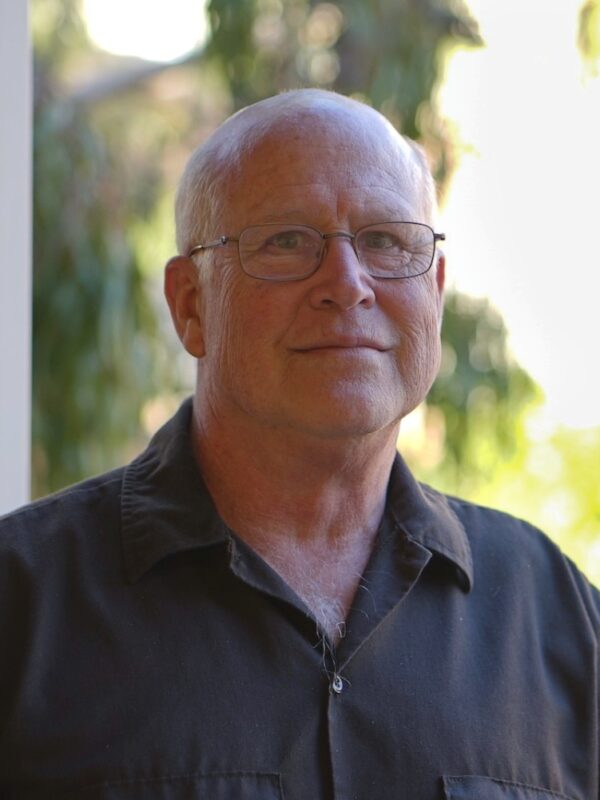 James C. McWilliams合作论文数Institute of the Environment & Sustainability, University of California, Los Angeles;Department of Atmospheric and Oceanic Sciences, University of California, Los Angeles;Nanjing University of Information Science & Technology3
 Alistair Adcroft合作论文数Princeton University;Geophysical Fluids Dynamics Laboratory, National Oceanic and Atmospheric Administration3
 Chris Horvat合作论文数Department of Physics, University of Auckland;Faculty of Science, University of Auckland;Climate Systems Laboratory, University of Auckland;Department of Earth, Environmental, and Planetary Sciences, Brown University3
 Peter Sullivan合作论文数National Center for Atmospheric Research3
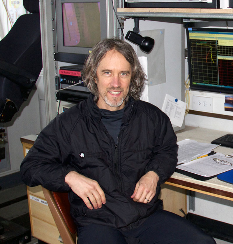 Stephen Matthew Griffies (Stephen M. Griffies)合作论文数Princeton University;Geophysical Fluid Dynamics Laboratory, National Oceanic and Atmospheric Administration3
 Robert Hallberg合作论文数Geophysical Fluid Dynamics Laboratory, National Oceanic and Atmospheric Administration;Princeton University3Ramsey R. Harcourt合作论文数3
 Amanda H. Lynch合作论文数Institute at Brown for Environment and Society, Brown University;Department of Earth, Environmental and Planetary Sciences, Brown University3
 Gokhan Danabasoglu合作论文数Oceanography Section, Climate and Global Dynamics Laboratory, National Science Foundation National Center for Atmospheric Research3a l m grant合作论文数2C Horvat合作论文数2
 z zheng合作论文数Appl Phys Lab, Univ Washington2Henry Chang合作论文数2
 Helene Theresa Hewitt合作论文数Met Off Hadley Ctr, Exeter, Devon, England2
 Qing Li合作论文数2A. D. Kirwan合作论文数2Andrew Poje合作论文数Division of Applied Mathematics, Brown University2
 William G. Large合作论文数Climate and Global Dynamics Division, National Center for Atmospheric Research2Tetsu Hara合作论文数Graduate School of Oceanography;University of Rhode Island;Graduate School of Oceanography, University of Rhode Island2
 Tom P. Rippeth合作论文数College of Natural Sciences, Bangor University2Helga Huntley合作论文数2Sarah W. Cooley合作论文数1D. A. Bailey合作论文数1w large合作论文数1E. Keenan合作论文数1
 Katherine M. Smith合作论文数1Sanchit Mehta合作论文数1Jean-Baptiste Sallée合作论文数1rr harcourt合作论文数1
 Daniel F. Carlson合作论文数1patrick orenstein合作论文数1Amrapalli Garanaik合作论文数Oregon State University1
 Leah Johnson合作论文数Dept Earth Environm & Planetary Sci, Brown Univ1
 Rachel Robey合作论文数Dept Appl Math, Univ Colorado1
 Gregory G. Garner合作论文数The, Pennsylvania State University1




