The surface energy budget (SEB) is a central regulator of Arctic climate and sea ice evolution, yet its processes remain poorly constrained due to sparse observations and complex, coupled surface-atmosphere interactions. This study leverages year-long measurements from the Multidisciplinary drifting Observatory for the Study of Arctic Climate (MOSAiC) to provide the most comprehensive assessment to date of the central Arctic SEB and its modulation by atmospheric variability. Ship-and ice-based observations from October 2019 to September 2020 were used to directly measure or tightly constrain each term of the SEB, leading to exceptional energetic closure with the seasonal snow and ice mass balance. The analysis reveals strong seasonal transitions in atmosphere-surface energy transfer that are modulated by the atmospheric state and constrained by the ability of the surface temperature to respond. Classification of the atmosphere into its two dominant radiative states-the semi-transparent (ST) and opaque (OP)-highlights the central role of synoptic-scale variability in clouds. The ST atmospheric state dominated the long winter ice growth season, with limited cloudiness supporting persistent surface radiative cooling and ice growth. The OP state, associated with liquid-containing or thick ice clouds, became dominant in spring, with the combination of increased solar heating and cloud surface longwave warming driving ice and snow melt. Eddy covariance versus bulk approaches for deriving surface turbulent heat fluxes provide vastly different perspectives on the role of turbulence in modulating the SEB. These results establish a high-quality benchmark dataset for Arctic SEB studies and demonstrate how the balance of atmospheric radiative states exerts a first-order control on the annual evolution of the sea ice. The findings have broad implications for advancing observing technologies, understanding Arctic amplification, improving climate models, and predicting future sea ice change.
Melt ponds are a common feature of the Arctic sea-ice environment during summer, and they play an important role in the exchange of heat and water vapor between the ocean and the atmosphere. We report the results of a time-series study of the CO2 dynamics within melt ponds (and nearby lead) and related fluxes with the atmosphere during the summer-to-autumn transition in the central Arctic Ocean during the Multidisciplinary drifting Observatory for the Study of Arctic Climate (MOSAiC) expedition. In late summer 2020, low-salinity meltwater was distributed throughout the melt ponds, and undersaturation of pCO2 in the meltwater drove a net influx of CO2 from the atmosphere. The meltwater layer subsequently thinned due to seawater influx, and a strong gradient in salinity and low-pCO2 water was observed at the interface between meltwater and seawater at the beginning of September. Mixing between meltwater and underlying seawater drives a significant drawdown of pCO2 as a result of the non-linearities in carbonate chemistry. By the middle of September, the strong stratification within the meltwater had dissipated. Subsequent freezing then began, and cooling and wind-induced drifting of ice floes caused mixing and an influx of seawater through the bottom of the melt pond. The pCO2 in the melt pond reached 300 µatm as a result of exchanging melt pond water with the underlying seawater. However, gas exchange was impeded by the formation of impermeable freshwater ice on the surface of the melt pond, and the net flux of CO2 was nearly zero into the pond, which was no longer a sink for atmospheric CO2. Overall, the melt ponds in this Arctic sea-ice area (both melt ponds and lead water) act as moderate sinks for atmospheric CO2.
Studying tropospheric ozone over the remote areas of the planet, such as the open oceans and the polar regions, is crucial to understand the role of ozone as a global climate forcer and regulator of atmospheric oxidative capacity. A focus on the pristine oceanic and polar regions complements the available land-based datasets and provides insights into key photochemical and depositional loss processes that control the concentrations and spatiotemporal variability in ozone as well as the physicochemical mechanisms driving these patterns. However, an assessment of the role of ozone over the oceanic and polar regions has been hampered by a lack of comprehensive observational datasets. Here, we present the first comprehensive collection of ozone data over the oceans and the polar regions. The overall dataset consists of 77 ship cruises/buoy-based observations and 48 aircraft-based campaigns. The dataset, consisting of more than 630 000 independent ozone measurement data points covering the period from 1977 to 2022 and an altitude range from the surface to 5000 m (with a focus on the lowest 2000 m), allows systematic analyses of the spatiotemporal distribution and long-term trends over the 11 defined ocean/polar regions. The datasets from ships, buoys, and aircraft are complemented by ozonesonde data from 29 launch sites or field campaigns and by 21 non-polar and 17 polar ground-based station datasets. The datasets contain information on how long the observed air masses were isolated from land, as estimated by backward trajectories from the individual observation points. To extract observations representative of oceanic conditions, we recommend using a subset of the data with an isolation time of 72 h or longer, from the analysis with coincident radon observations. These filtered oceanic and polar data showed typically flat diurnal cycles at high latitudes, whereas daytime decreases in ozone (11 %-16 %) were observed at lower latitudes. The ship/buoy- and aircraft-based datasets presented here will supplement the land-based ones in the TOAR-II (Tropospheric Ozone Assessment Report Phase II) database to provide a fully global assessment of tropospheric ozone. The described dataset is available at 10.17596/0004044 (Kanaya et al., 2025).
Direct measurements using eddy covariance methodology of turbulent heat and momentum fluxes were observed from the Met City tower during MOSAiC. In models, these fluxes are parameterized using bulk aerodynamic algorithms for which the transfer coefficients must be found. In practice, the coefficients are constrained iteratively to resolve the co-dependence between Obukhov Length (necessary for calculating the coefficients) and the friction velocity, u* (an expression of the Reynold’s stress solved for by the algorithm). The aerodynamic roughness length, z0, is also needed to calculate the coefficients. For calculations over the global ocean, z0 is coupled to the atmosphere through u*. However, over sea ice the meteorological correlation is weak and the physical surface roughness is heterogeneous and decoupled from the atmosphere. This introduces a vulnerability into the calculation and necessitates assumptions about z0. At MOSAiC, the tower measurements of z0 show an evolution from early- to late-winter of nearly 2 orders of magnitude where 1 order nominally corresponds to a 30-40% differences in the derived fluxes. In this presentation we evaluate the error in bulk calculations due to the z0 assumption to assess what could be gained from a surface aware scheme.
Abstract. Studying tropospheric ozone over the remote areas of the planet, such as the open oceans and the polar regions, is crucial to understand the role of ozone as a global climate forcer and regulator of atmospheric oxidative capacity. A focus on the pristine oceanic and polar regions complements the available land-based data sets and provides insights into key photochemical and depositional loss processes that control the concentrations, spatio-temporal variability of ozone, and the physico-chemical mechanisms driving these patterns. However, an assessment of the role of ozone over the oceanic and polar regions has been hampered by a lack of comprehensive observational data sets. Here, we present the first comprehensive collection of ozone data over the oceans and the polar regions. The overall data set consists of 77 ship cruises/buoy-based observations and 48 aircraft-based campaigns. The data set, consisting of more than 630,000 independent ozone measurement data points covering the period from 1977 to 2022 and an altitude range from the surface to 5000 m (with a focus on the lowest 2000 m), allows systematic analyses of the spatio-temporal distribution and long-term trends over the defined 11 ocean/polar regions. The data sets from ships, buoys, and aircrafts are complemented with an ozonesonde data set from 29 launch sites or field campaigns, and by 21 non-polar and 17 polar ground-based stations data sets. The data were filtered by using backward trajectories calculated with the HYSPLIT model from the individual observation points to extract essentially oceanic observations, defined as air masses that have travelled over oceans for 72 hours or more, which were further tested with the coincident Radon observations. The oceanic and polar data thus selected showed typically flat diurnal patterns at high latitudes and daytime decreases (11–16 %) at low latitudes, indicating the adequacy of the data collection and processing procedures, as well as the potential for further studies of processes with statistical robustness and coverage. The ship/buoy- and aircraft-based data sets presented here will supplement the land-based ones in the TOAR-II database to provide a fully global assessment of tropospheric ozone.
Photochemical release of iodine from snow has been suggested as a source of reactive iodine to the Arctic atmosphere, however understanding of the underlying mechanism and potential source strength is hindered by a lack of measurements of iodine concentration and speciation in snow. Moreover, the origin of snow iodine is also unknown. Here, we report iodine speciation measurements in Arctic snow on sea ice at a range of snow depths from 177 samples, representing 80 sampling events, from December 2019 to October 2020 collected during the Multidisciplinary drifting Observatory for the Study of Arctic Climate (MOSAiC) expedition. We demonstrate that while there appears to be a source of iodine, in particular iodate, to the base of the snow over first year ice, this does not influence iodine concentration in the surface snow. There is instead evidence of a top-down source of iodine, potentially from iodine-enriched marine aerosol, as well as some evidence for episodic influx of iodate with dust. The potential for photochemical release of molecular iodine (I2) from iodide in surface snow was investigated, and it was demonstrated that this could provide an iodine emission flux to the Arctic atmosphere comparable to oceanic fluxes. Knowledge of the prevalence and speciation of iodine in Arctic snow will contribute to better understanding of its contribution to observed concentrations of polar iodine oxide (IO), and hence its contribution to the depletion of tropospheric ozone in the Arctic.
This study presents the application of generative deep learning techniques to evaluate marine fog visibility nowcasting using the FATIMA (Fog and turbulence interactions in the marine atmosphere) campaign observations collected during July 2022 in the North Atlantic in the Grand Banks area and vicinity of Sable Island (SI), northeast of Canada. The measurements were collected using the Vaisala Forward Scatter Sensor model FD70 and Weather Transmitter model WXT50, and Gill R3A ultrasonic anemometer mounted on the Research Vessel Atlantic Condor. To perform nowcasting, the time series of fog visibility (Vis), wind speed, dew point depression, and relative humidity with respect to water were preprocessed to have lagged time step features. Generative nowcasting of Vis time series for lead times of 30 and 60 minutes were performed using conditional generative adversarial networks (cGAN) regression at visibility thresholds of Vis < 1 km and < 10 km. Extreme gradient boosting (XGBoost) was used as a baseline method for comparison against cGAN. At the 30 min lead time, Vis was best predicted with cGAN at Vis < 1 km (RMSE = 0.151 km) and with XGBoost at Vis < 10 km (RMSE = 2.821 km). At the 60 min lead time, Vis was best predicted with XGBoost at Vis < 1 km (RMSE = 0.167 km) and Vis < 10 km (RMSE = 3.508 km), but the cGAN RMSE was similar to XGBoost. Despite nowcasting Vis at 30 min being quite difficult, the ability of the cGAN model to track the variation in Vis at 1 km suggests that there is potential for generative analysis of marine fog visibility using observational meteorological parameters.
Introduction: This study presents the application of machine learning (ML) to evaluate marine fog visibility conditions and nowcasting of visibility based on the FATIMA (Fog and turbulence interactions in the marine atmosphere) campaign observations collected during July 2022 in the North Atlantic in the Grand Banks area and vicinity of Sable Island, northeast of Canada.Methods: The measurements were collected using instrumentation mounted on the Research Vessel Atlantic Condor. The collected meteorological parameters were: visibility (Vis), precipitation rate, air temperature, relative humidity with respect to water, pressure, wind speed, and direction. Using all variables, the droplet number concentration was used to qualitatively indicate and assess characteristics of the fog using the t-distributed stochastic neighbor embedding projection method (t-SNE), which clustered the data into groups. Following t-SNE analysis, a correlation heatmap was used to select relevant meteorological variables for visibility nowcasting, which were wind speed, relative humidity, and dew point depression. Prior to nowcasting, the input variables were preprocessed to generate additional time-lagged variables using a 120-minute lookback window in order to take advantage of the intrinsic time-varying features of the time series data. Nowcasting of Vis time series for lead times of 30 and 60 minutes was performed using the ML regression methods of support vector regression (SVR), least-squares gradient boosting (LSB), and deep learning at visibility thresholds of Vis < 1 km and < 10 km.Results: Vis nowcasting at the 60 min lead time was best with LSB and was significantly more skillful than persistence analysis. Specifically, using LSB the overall nowcasts at Vis 1 < km and Vis 10 < km were RMSE = 0.172 km and RMSE = 2.924 km, respectively. The nowcasting skill of SVR for dense fog (Vis ≤ 400 m) was significantly better than persistence at all Vis thresholds and lead times, even when it was less skillful than persistence at predicting high visibility.Discussion: Thus, ML techniques can significantly improve Vis prediction when either observations or modelbased accurate time-dependent variables are available. The results suggest that there is potential for future ML analysis that focuses on modeling the underlying factors of fog formation.
In the central Arctic, warm and moist air intrusions (WAMIs) are increasingly prevalent during winter and spring, significantly impacting the near-surface energy budget. This study investigates WAMI-induced transport and wet deposition of black carbon (BC) and its subsequent influence on snow properties and melting. Using a modeling approach combined with extensive observational data from the 2019–2020 Multidisciplinary drifting Observatory for the Study of Arctic Climate (MOSAiC) expedition, we document several episodes of elevated BC wet deposition during winter and spring (Nov–Apr). These events, driven by WAMI-transported pollution and moisture, result in an average 41% increase in BC wet deposition compared to typical winter/spring conditions. Furthermore, this enhanced BC deposition contributes to increased solar energy absorption (+3.4–4.6 W/m2 on average) and accelerated snowpack melt rate (+24–36%) during the subsequent summer. Despite their episodic occurrence (only 15% of the time), this study underscores the critical role of WAMIs in shaping the central Arctic environment and emphasizes the importance of the BC snow albedo effect. Our findings highlight the need for further investigation into the broader climatic impacts of WAMI-induced pollution transport in the Arctic.
The Multidisciplinary drifting Observatory for the Study of Arctic Climate (MOSAiC) was a yearlong expedition supported by the icebreaker R/V Polarstern, following the Transpolar Drift from October 2019 to October 2020. The campaign documented an annual cycle of physical, biological, and chemical processes impacting the atmosphere-ice-ocean system. Of central importance were measurements of the thermodynamic and dynamic evolution of the sea ice. A multi-agency international team led by the University of Colorado/CIRES and NOAA-PSL observed meteorology and surface-atmosphere energy exchanges, including radiation; turbulent momentum flux; turbulent latent and sensible heat flux; and snow conductive flux. There were four stations on the ice, a 10 m micrometeorological tower paired with a 23/30 m mast and radiation station and three autonomous Atmospheric Surface Flux Stations. Collectively, the four stations acquired ~928 days of data. This manuscript documents the acquisition and post-processing of those measurements and provides a guide for researchers to access and use the data products.
The rapid melt of snow and sea ice during the Arctic summer provides a significant source of low-salinity meltwater to the surface ocean on the local scale. The accumulation of this meltwater on, under, and around sea ice floes can result in relatively thin meltwater layers in the upper ocean. Due to the small-scale nature of these upper-ocean features, typically on the order of 1 m thick or less, they are rarely detected by standard methods, but are nevertheless pervasive and critically important in Arctic summer. Observations during the Multidisciplinary drifting Observatory for the Study of Arctic Climate (MOSAiC) expedition in summer 2020 focused on the evolution of such layers and made significant advancements in understanding their role in the coupled Arctic system. Here we provide a review of thin meltwater layers in the Arctic, with emphasis on the new findings from MOSAiC. Both prior and recent observational datasets indicate an intermittent yet long-lasting (weeks to months) meltwater layer in the upper ocean on the order of 0.1 m to 1.0 m in thickness, with a large spatial range. The presence of meltwater layers impacts the physical system by reducing bottom ice melt and allowing new ice formation via false bottom growth. Collectively, the meltwater layer and false bottoms reduce atmosphere-ocean exchanges of momentum, energy, and material. The impacts on the coupled Arctic system are far-reaching, including acting as a barrier for nutrient and gas exchange and impacting ecosystem diversity and productivity.
Understanding the mercury cycle in the Arctic is important due to the harmful bioaccumulation of its toxic form, methylmercury, in wildlife and ultimately Arctic residents. Gaseous elemental mercury (Hg(0)) is relatively well-mixed across the northern hemisphere atmosphere due to its long atmospheric lifetime. Hg(0) can be oxidized, especially in the Arctic spring during halogen-driven depletion events. The resulting gaseous oxidized mercury (Hg(II)) is relatively quickly deposited onto snow, either directly or via condensing onto particles, forming particulate mercury (PHg). It is generally understood that a large fraction of the deposited Hg(II) and PHg is photoreduced to Hg(0) and re-emitted to the atmosphere. However, mercury remaining in the snowpack till melt can become bioavailable through entering the ocean.There is a severe lack of Hg(II) and PHg observations in the central Arctic, particularly over sea ice, limiting our understanding of the mercury cycle in that region and inhibiting us from quantifying mercury budgets in all environmental compartments and particularly where it unfolds its harmful neurotoxic effects. Moreover, most of the observational efforts aiming at creating process understanding focused on spring during mercury depletion events or the snow melt period, leaving large knowledge gaps for fall and winter.Here, we show atmospheric observations of PHg during MOSAiC, measured with an aerosol mass spectrometer in fall and spring over the central Arctic pack ice. In both seasons, PHg concentrations correlate strongly with wind speed and chloride, suggesting a mechanical (wind-driven) process behind atmospheric PHg related partly to blowing snow. In addition, there are significant differences between fall and spring observations (e.g. no atmospheric mercury depletion events in fall), suggesting that various processes are at play.This wind-driven process has hitherto not been reported and is different from observations at land-based stations as well as previous measurements over sea ice that ascribed the formation of PHg to adsorption of Hg(II) onto pre-existing aerosols or diamond dust rather than aerosolization from the snow pack. We hypothesize, based on snow chemical analyzes and literature, that the elevated halide content in snow on sea ice creates complexes of PHg, which are much harder to photoreduce than Hg(II), leading to a larger PHg content in snow. These processes of forming PHg and wind-driven aerosolization have implications for the mercury content of snow and the distances over which PHg is re-deposited after atmospheric transport given that the lifetime of PHg is about one order of magnitude larger than that of Hg(II) in the atmosphere.
Dry deposition to the surface is one of the main removal pathways of tropospheric ozone (O3). We quantified for the first time the impact of O3 deposition to the Arctic sea ice on the planetary boundary layer (PBL) O3 concentration and budget using year-round flux and concentration observations from the Multidisciplinary drifting Observatory for the Study of Arctic Climate (MOSAiC) campaign and simulations with a single-column atmospheric chemistry and meteorological model (SCM). Based on eddy-covariance O3 surface flux observations, we find a median surface resistance on the order of 20,000 s m−1, resulting in a dry deposition velocity of approximately 0.005 cm s−1. This surface resistance is up to an order of magnitude larger than traditionally used values in many atmospheric chemistry and transport models. The SCM is able to accurately represent the yearly cycle, with maxima above 40 ppb in the winter and minima around 15 ppb at the end of summer. However, the observed springtime ozone depletion events are not captured by the SCM. In winter, the modelled PBL O3 budget is governed by dry deposition at the surface mostly compensated by downward turbulent transport of O3 towards the surface. Advection, which is accounted for implicitly by nudging to reanalysis data, poses a substantial, mostly negative, contribution to the simulated PBL O3 budget in summer. During episodes with low wind speed (<5 m s−1) and shallow PBL (<50 m), the 7-day mean dry deposition removal rate can reach up to 1.0 ppb h−1. Our study highlights the importance of an accurate description of dry deposition to Arctic sea ice in models to quantify the current and future O3 sink in the Arctic, impacting the tropospheric O3 budget, which has been modified in the last century largely due to anthropogenic activities.
Near-surface mercury and ozone depletion events occur in the lowest part of the atmosphere during Arctic spring. Mercury depletion is the first step in a process that transforms long-lived elemental mercury to more reactive forms within the Arctic that are deposited to the cryosphere, ocean, and other surfaces, which can ultimately get integrated into the Arctic food web. Depletion of both mercury and ozone occur due to the presence of reactive halogen radicals that are released from snow, ice, and aerosols. In this work, we added a detailed description of the Arctic atmospheric mercury cycle to our recently published version of the Weather Research and Forecasting model coupled with Chemistry (WRF-Chem 4.3.3) that includes Arctic bromine and chlorine chemistry and activation/recycling on snow and aerosols. The major advantage of our modelling approach is the online calculation of bromine concentrations and emission/recycling that is required to simulate the hourly and daily variability of Arctic mercury depletion. We used this model to study coupling between reactive cycling of mercury, ozone, and bromine during the Multidisciplinary drifting Observatory for the Study of Arctic Climate (MOSAiC) spring season in 2020 and evaluated results compared to land -based, ship-based, and remote sensing observations. The model predicts that elemental mercury oxidation is driven largely by bromine chemistry and that particulate mercury is the major form of oxidized mercury. The model predicts that the majority (74%) of oxidized mercury deposited to land-based snow is re-emitted to the atmosphere as gaseous elemental mercury, while a minor fraction (4%) of oxidized mercury that is deposited to sea ice is re-emitted during spring. Our work demonstrates that hourly differences in bromine/ozone chemistry in the atmosphere must be considered to capture the springtime Arctic mercury cycle, including its integration into the cryosphere and ocean.
Atmospheric gaseous elemental mercury (GEM) concentrations in the Arctic exhibit a clear summertime maximum, while the origin of this peak is still a matter of debate in the community. Based on summertime observations during the Multidisciplinary drifting Observatory for the Study of Arctic Climate (MOSAiC) expedition and a modeling approach, we further investigate the sources of atmospheric Hg in the central Arctic. Simulations with a generalized additive model (GAM) show that long-range transport of anthropogenic and terrestrial Hg from lower latitudes is a minor contribution (~2%), and more than 50% of the explained GEM variability is caused by oceanic evasion. A potential source contribution function (PSCF) analysis further shows that oceanic evasion is not significant throughout the ice-covered central Arctic Ocean but mainly occurs in the Marginal Ice Zone (MIZ) due to the specific environmental conditions in that region. Our results suggest that this regional process could be the leading contributor to the observed summertime GEM maximum. In the context of rapid Arctic warming and the observed increase in width of the MIZ, oceanic Hg evasion may become more significant and strengthen the role of the central Arctic Ocean as a summertime source of atmospheric Hg.
Chlorine radicals are strong atmospheric oxidants known to play an important role in the depletion of surface ozone and the degradation of methane in the Arctic troposphere. Initial oxidation processes of chlorine produce chlorine oxides, and it has been speculated that the final oxidation steps lead to the formation of chloric (HClO 3 ) and perchloric (HClO 4 ) acids, although these two species have not been detected in the atmosphere. Here, we present atmospheric observations of gas-phase HClO 3 and HClO 4 . Significant levels of HClO 3 were observed during springtime at Greenland (Villum Research Station), Ny-Ålesund research station and over the central Arctic Ocean, on-board research vessel Polarstern during the Multidisciplinary drifting Observatory for the Study of the Arctic Climate (MOSAiC) campaign, with estimated concentrations up to 7 × 10 6 molecule cm −3 . The increase in HClO 3 , concomitantly with that in HClO 4 , was linked to the increase in bromine levels. These observations indicated that bromine chemistry enhances the formation of OClO, which is subsequently oxidized into HClO 3 and HClO 4 by hydroxyl radicals. HClO 3 and HClO 4 are not photoactive and therefore their loss through heterogeneous uptake on aerosol and snow surfaces can function as a previously missing atmospheric sink for reactive chlorine, thereby reducing the chlorine-driven oxidation capacity in the Arctic boundary layer. Our study reveals additional chlorine species in the atmosphere, providing further insights into atmospheric chlorine cycling in the polar environment.
Unlike bromine, the effect of iodine chemistry on the Arctic surface ozone budget is poorly constrained. We present ship-based measurements of halogen oxides in the high Arctic boundary layer from the sunlit period of March to October 2020 and show that iodine enhances springtime tropospheric ozone depletion. We find that chemical reactions between iodine and ozone are the second highest contributor to ozone loss over the study period, after ozone photolysis-initiated loss and ahead of bromine.
The bubbles generated by breaking waves are of considerable scientific interest due to their influence on air–sea gas transfer, aerosol production, and upper ocean optics and acoustics. However, a detailed understanding of the processes creating deeper bubble plumes (extending 2–10 m below the ocean surface) and their significance for air–sea gas exchange is still lacking. Here, we present bubble measurements from the HiWinGS expedition in the North Atlantic in 2013, collected during several storms with wind speeds of 10–27 m s−1. A suite of instruments was used to measure bubbles from a self-orienting free-floating spar buoy: a specialised bubble camera, acoustical resonators, and an upward-pointing sonar. The focus in this paper is on bubble void fractions and plume structure. The results are consistent with the presence of a heterogeneous shallow bubble layer occupying the top 1–2 m of the ocean, which is regularly replenished by breaking waves, and deeper plumes which are only formed from the shallow layer at the convergence zones of Langmuir circulation. These advection events are not directly connected to surface breaking. The void fraction distributions at 2 m depth show a sharp cut-off at a void fraction of 10−4.5 even in the highest winds, implying the existence of mechanisms limiting the void fractions close to the surface. Below wind speeds of 16 m s−1 or a wind-wave Reynolds number of RHw=2×10⁶, the probability distribution of void fraction at 2 m depth is very similar in all conditions but increases significantly above either threshold. Void fractions are significantly different during periods of rising and falling winds, but there is no distinction with wave age. There is a complex near-surface flow structure due to Langmuir circulation, Stokes drift, and wind-induced current shear which influences the spatial distribution of bubbles within the top few metres. We do not see evidence for slow bubble dissolution as bubbles are carried downwards, implying that collapse is the more likely termination process. We conclude that the shallow and deeper bubble layers need to be studied simultaneously to link them to the 3D flow patterns in the top few metres of the ocean. Many open questions remain about the extent to which deep bubble plumes contribute to air–sea gas transfer. A companion paper (Czerski et al., 2022) addresses the observed bubble size distributions and the processes responsible for them.
 Barry Huebert合作论文数Department of Oceanography, University of Hawai`i at Manoa46
 Chris Fairall合作论文数Physical Science Division, Earth Systems Research Laboratory, National Oceanic and Atmospheric Administration;Physical Sciences Laboratory, National Oceanic and Atmospheric Administration40
 Alan R. Bandy合作论文数31
 Stephen D. Archer合作论文数Plymouth Marine Laboratory18
 Ming-Xi Yang合作论文数Plymouth Marine Laboratory16
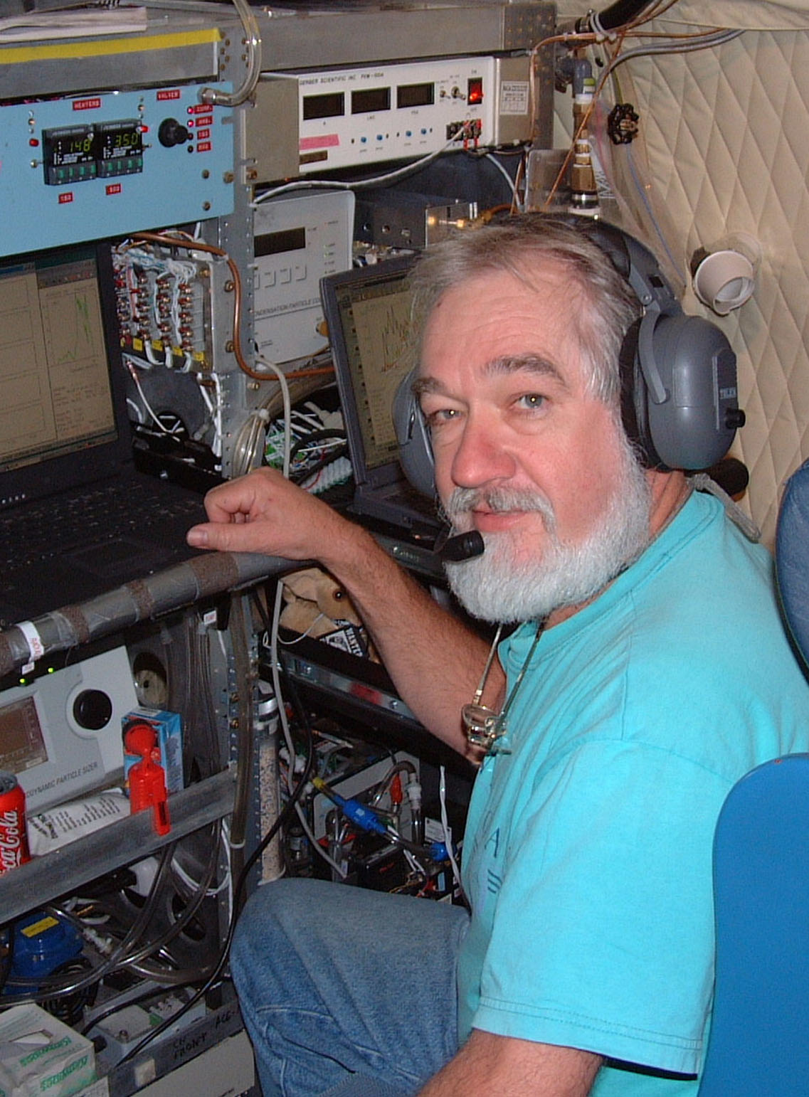 Antony Clarke合作论文数Department of Oceanography, School of Ocean & Earth Science & Technology, University of Hawai`i at Manoa14Steven G. Howell合作论文数School of Ocean, Earth Science and Technology, University of Hawaii14
 Ludovic Bariteau合作论文数13Donald C Thornton合作论文数13Donald C. Thornton合作论文数12ian m brooks合作论文数11
 Helene Angot合作论文数Extreme Environm Res Lab, Ecole Polytech Fed Lausanne EPFL11
 Ivo Beck合作论文数11
 Julia Schmale合作论文数School of Architecture, Civil and Environmental Engineering, École Polytechnique Fédérale de Lausanne11
 Harindra Joseph Fernando合作论文数Environmental Fluid Mechanics Laboratory, College of Engineering, University of Notre Dame;Arizona State University10
 Andrey A. Grachev合作论文数Atmospheric Dynamics & Analytics Branch, US Army Research Laboratory10
 P. Ola G. Persson合作论文数10
 Dean Howard合作论文数9Lauriane L. J. Quéléver合作论文数9Tiia Laurila合作论文数9
 Kevin Posman合作论文数9
 Tuija Jokinen合作论文数Department of Physics, University of Helsinki;Department of Physics, University of Helsinki9
 Philip D Nightingale合作论文数Plymouth Marine Laboratory9
 Detlev Helmig合作论文数Institute of Arctic and Alpine Research, University of Colorado Boulder9
 Matthew Shupe合作论文数NOAA Physical Sciences Laboratory;Cooperative Institute for Research in Environmental Sciences, University of Colorado9Timothy H. Bertram合作论文数8Hans-Werner Jacobi合作论文数8Matthew Boyer合作论文数7
 Rodney Weber合作论文数School of Earth and Atmospheric Sciences, College of Sciences, Georgia Institute of Technology7
 Laura S. Leo合作论文数7
 Madison Smith合作论文数Appl Phys Lab, Univ Washington6
 Robin W. Pascal合作论文数National Oceanography Centre6
 Ian C. Faloona合作论文数Department of Land, Air and Water Resources, University of California, Davis6C. S. McNaughton合作论文数6j e hare合作论文数5
 Sophia E Brumer合作论文数Ocean & Climate Phys Div, Columbia Univ5
 Tuukka Petäjä合作论文数Institute for Atmospheric and Earth System Research, Faculty of Science, University of Helsinki5
 Jim M. Thomson合作论文数Applied Physics Laboratory, Department of Civil & Environmental Engineering, College of Engineering, University of Washington5
 Donald H. Lenschow (Don Lenschow)合作论文数Mesoscale and Microscale Meteorology Laboratory, National Center for Atmospheric Research5J. Kline合作论文数5
 Timothy S. Bates合作论文数College of the Environment, University of Washington5Wolfgang Nadler合作论文数5
 Jacques Hueber合作论文数5P. S. Guest合作论文数4Adam J Christman合作论文数4Christopher M. Hocut合作论文数Army Res Lab, DEVCOM4
 Helen Czerski合作论文数Department of Mechanical Engineering, University College London4
 Christopher Richard Cox合作论文数4
 Gregory Carmichael合作论文数Department of Chemical & Biochemical Engineering, University of Iowa4




